
斯坦福 CS221 人工智能导论笔记(二)
Okay。Okay。Okay。Okay。(mumbling)。Yeah。Right。Okay。Okay。or two。Okay。Okay。Okay。Yeah。Okay。Okay。Okay。Okay。Okay。okay?Yeah。Yeah。okay?- Yeah。- Great。Thanks。Right?Okay?Okay?Okay?Okay。Okay?Okay?Okay?Okay?
P14:Lecture 14 Bayesian Networks 2 - Forward-Backward - 鬼谷良师 - BV16E411J7AQ
All right, let’s get started。
So we’re going to continue talking about Bayesian networks。
which we started on Monday。 And just a quick recap, we’ve been talking about Bayesian networks。 which is a new paradigm for defining models。 And what is a Bayesian network?
You have a set of variables, which are nodes in a graph。 For example, whether you have a cold。 whether you have allergies, where you’re coughing, whether you have HEIs。 These nodes are related by a set of directed edges, which capture various dependencies。 For example。 HEIs is caused by allergies, but not cold or by cough。 And then formally。
for every variable in the Bayesian network, you have a local conditional distribution。 which specifies the distribution over that variable, given the parents。 So the parents of cough are cold and allergies。 So you would have a local conditional distribution。 of P of H given CNA。 You do that for all the variables。 And finally, you take all the factors。
or local conditional distributions, and multiply them together。 And you can one glorious joint distribution, over all the possible variables in your distribution。 So in other words, to sum it up, you can think about Bayesian networks。 as factor graphs plus probability。 They allow you to define, ginormous joint distributions。
over lots of random variables, using factor graphs。 which allow you to specify things very compactly。 And moreover, we saw glimpses。 of how we can use the structure of factor graphs, to permit efficient inference。 So probabilistic inference in Bayesian networks, is the task of given a Bayesian network。
which is this oracle about what you know about the world。 And you look at some evidence that you’ve found。 So it’s raining or not raining。 or you have HEIs or so on。 And you condition on that evidence。 and you also have a set of query variables, that you’re interested in asking about。
And the goal is to compute, the probability of the query variables。 conditioned on the evidence that you see。 Big E equals little E。 Remember, lower upper case is。 random variables lower case is actual values。 And so for example, in the coughing case。 there’s the probability of a cold, given the fact that you’re coughing, but don’t have HEIs。
And this probability is defined, by just the laws of probability。 which we went over the first slide of last lecture。 And the challenge is how to do this efficiently。 Okay, and that’s gonna be the topic of this class。 So any questions about the basic setup。 of what Bayesian networks are, and how do you, what does mean to do probabilistic inference? Okay。
one maybe kind of a high level note, about Bayesian networks is that。 I think they’re really powerful as a way, to describe kind of knowledge。 I think a lot of AI today is focused on particular tasks。 where you define some input and you define some output, and you train a classifier。
And the classifier that you train, can only do this one thing, input output。 But the paradigm behind Bayesian networks, and databases in general is that。 you have developed a kind of a knowledge source, which can be probabilistic。 It’s captured by this joint distribution。 And once you have it。
you use all the tools of probability, to allow you to answer arbitrary questions about it。 So you can give me any pieces of evidence and any query, and it’s clear what I’m meant to do。 I’m supposed to compute these values。 So it’s kind of a more flexible and powerful paradigm。 than just converting inputs to outputs。 And so that’s why I think it’s so interesting。 Okay。
so today we’re gonna focus on, how to compute these arbitrary inference queries efficiently。 I’m gonna start with forward, backward and particle filtering。 These are going to specialize。 to the specific Bayesian networks called HMMs, hidden Markov models。 And then we’re gonna look at Gibbs sampling, which is a much more general way of doing things。 Okay。
so a hidden Markov model, which I talked about last time。 which we’re going to go in more detail this time, is a Bayesian network where there exists。 a sequence of hidden variables, and a corresponding sequence of observed variables。 So as a kind of motivating example, imagine you’re tracking some sort of object, in your homework。
you’ll be tracking cars。 So H_i is going to be the location of the object or car。 at a particular time step i。 And E_i is going to be some sort of sensor reading。 that you get at that particular time step。 It could be the location plus some noise。 or some sort of distance to that, the true object and so on。 Okay, so these are the variables。
And it goes well as saying that the hidden variables。 are hidden and observed variables are observed。 So the distributions over this。 all the variables is specified by three types, of local conditional distributions。 The first one is just the starting distribution。 What is the probability of H_1?
This could be a uniform over all possible locations, just as an example。 And then we have the transition distributions, which specify what is the distribution。 over a particular hidden variable, the location of the true location of object, H_i。 given H_i minus one。 So this captures dynamics of how this object, or car might move over time。
For example, it could just be a uniform, over adjacent locations。 So cars can’t teleport。 they can only move to adjacent locations, over a one time step。 And finally。 we have emission distributions, which govern how the sensor reading。 is computed as a function of the location。 So this again could be something as simple。
as uniform over adjacent locations。 If you expect to see some noise in your sensor。 the sensor doesn’t tell you where exactly the car is, but tells you approximately where the car is。 And the joint distribution over all these random variables。 is going to be given by simply the product, of everything you see on the board。
I’m just gonna write this up on the board, just for reference。 So we have the probability of H equals H。 So this, when I write H equals H。 that means the H_1 through H_n。 So all the random variables, all the hidden random variables。 all the observed random variables。 And this is my definition equal to, the start distribution。
Let’s see, just make sure I have, okay, good notation here。 So start distribution over H_1。 And then I have the transitions, I equals one, I guess, two to n, just to make sure, okay。 So this is the probability of H_i given H_i minus one。 And then finally, I have for every time step。 I through one through n, I have the probability of observation given H_i。
So multiply all these factors together。 That gives me a single number that is the probability。 of all the observed and all the hidden variables。 Any questions about the definition of a hidden Markov model?
Okay, so given we have one of these models, remember with a Bayesian network。 I can answer any sort of queries。 I can ask what is the probability of H_3 given H_2 and E_5。 And I can do all sorts of crazy things。 And all of these things are possible and efficient。 you know, compute。 But we’re gonna focus on two main types of questions。 Motivated by the。
let’s say, object tracking, for example。 The first question is filtering。 Filtering says you’re at a particular time step, let’s say time step three。 What do I know about the true object location H_3, given all the evidence I’ve seen up until now?
So this is kind of a real time object tracking。 At each point in time, you look at all the evidence。 and you want to know where the object is。 A similar question is smoothing。 And you’re still looking at a particular time step, three, let’s say, but you’re conditioning。 on all the evidence。 So you’re looking at all the observations, and you’re looking at。
you’re kind of thinking about, this more retrospectively, where was the object, at time step three?
So think about if you’re trying to reconstruct, the trajectory or something。 Okay。 so this is called filtering and smoothing。 So let’s now try to develop an algorithm。 for answering these type of queries。 And without loss of generality。 I’m going to focus on answering smoothing queries。 So why is it the case that if I tell you。
I can solve all smoothing questions, I can also solve all filtering questions。 (mumbling)。 So it is true, so in filtering, this is the evidence is a subset。 But the answers are going to be different, depending on what evidence you compute on。 So you can’t literally just use one, as the answer for the other。 Yeah。
- It relies over the things that you, like E45 to get to。 - Yeah, so you marginalize。 That’s a key idea。 Is that suppose I had a smoother, and I wanted to answer this filtering query。 So this is H3 given E1 to E2, E3。 Remember last time we talked about how。 if you can take leaves of vision networks, which are not observed and just essentially wipe them away。
So if you don’t observe E4, E5, H4, H5, you can just pretend those things don’t exist。 Right。 And now you’re back to a smoothing query, where you’re conditioning on all the evidence。 Okay。 so we’re gonna focus on smoothing。 And to make a progress on this problem。 I’m going to introduce a representation, that’s gonna help us think about, the possible assignments。
Right, and just to be clear, right? There’s, the reason why this is not completely trivial。 is that there are, if you have end hidden variables, there’s two to end or X management。 and number of possible assignments, and you can’t just enumerate all of them。 So you’re gonna have to come up with some algorithm, that can compute it more efficiently。 Okay。
so what we’re gonna do is introduce, this latest representation。 which is gonna give us a compact way, of representing those assignments。 And then we can see how we can operate on that representation。 Okay, so this is gonna smell a lot。 like state-based model。 So we’re kind of going backwards, about, hopefully it’ll make sense。
So the idea behind a lattice representation, is that I’m going to have a set of rows and columns。 So each column is going to correspond, to a particular variable。 So the first column is gonna correspond to H1, and each row is gonna correspond。 to some setting of that variable。 So there’s two possible things I can do。
I can either set H1 equals one, or I can set H1 equals two。 The version I’m drawing on the board。 is gonna be a simplification of what I have on the slides, just in the interest of space。 And the second column is going to be either, H2 equals one, or H2 equals two。 So by going through these lattice nodes, which are drawn as boxes。
I’m kind of assigning random variables, to a particular value。 Okay, so I’m gonna connect these up。 So from this state, I can either set H2 equals one, or two。 Here I can also go from two, one。 or two。 And finally, let’s just do H3 equals one, H3 equals two。 And similarly。 I can choose either one of them, from no matter where I am。 And finally, I have an N state。 Okay。
So first, notice that the size of the lattice, is reasonably well controlled。 It’s simply the number of time steps, times the number of values that a variable can take on。 So let’s suppose that there’s N time steps。 And K possible, let’s say, locations, so values of HI。 So how many nodes are here? - Eight times N。 - Eight times N。 - Eight times N, right? Okay。
So that means we can, essentially, this doesn’t blow up exponentially。 Okay。 so now let us interpret a path from start to end。 What is a path from start to end tell us?
So let’s take this path。 Now, what does this tell us? Yeah。 - Particular assignment of a variable?
- Yeah, it’s a particular assignment of the variable。 So this one says set H1 to one, H2 to one。 H3 to one。 This path says set H1 to two, H1 to one, and H3 to two, and so on。 Okay。 So every path from start to end, is an assignment to all of the unobserved, or hidden variables。 Okay。 So now, remember, each assignment comes, with some sort of probability。
So we’re gonna try to represent those probabilities, juxtapose on this graph。 Okay。 so I’m gonna go through each of these edges。 So remember, these are the probabilities, right?
So every assignment is a product of the factors, and I’m going to basically take these factors。 and just sprinkle them on the edges, at the points where I can compute the factors。 and I’ll explain more what I mean by this。 Okay。 So maybe one kind of preliminary thing I should mention is。 suppose for this example, we have, we are conditioning on E1 equals one, E2 equals two。
let’s say E1 equals, sorry, E3 equals one。 Okay。 So I’m conditioning on these things。 Notice I’m not drawing them in here, because these are observed variables。 I don’t have to reason about what values they take on。 I’m only gonna consider the hidden variables。 which I don’t know。 But this is just gonna be some sort of reference。 Okay。
so let’s start with start to H1 equals one, right? So if you remember backtracking and CSPs, right。 we basically took factors, and then whenever we could evaluate the factor。 we just put it down on that edge in the backtracking tree。 So here, what can we do?
We have the probability of H1 equals one。 Okay。 And then we also have the probability。 of the first emission probability I can compute, right?
So that’s a probability of E1 equals the evidence I saw, which is one, given H1 equals one。 which is the value that I’ve committed to here。 So this is a number that is essentially the weight。 or cost or score or whatever you wanna call it, that I am going to incur when I traverse that edge。 Okay, so what about this one? So I have the transition from P, let’s say, H2 equals one。
given H1 equals one, and times the probability of E2 equals whatever I observe, which is two。 given H2 equals one。 And similarly, over here, I have probability of H3 equals one。 given H2 equals one, times the probability of E3 equals one, which is whatever I observe。 given H3 equals one。 And then over here, there’s no more factors left。
so I’m just gonna put one there。 Okay, so you can check that, when I traverse this path。 and then multiply all of these probabilities together。 that’s exactly this expression for H1 equals one, H2 equals one, H3 equals one, E1 equals one。 E2 equals two, E3 equals one。 And for each of these edges, I have an analogous quantity。
depending on the values that I’m dealing with。 Okay, any questions about this basic idea?
So in the slides, this is basically what I just said。 Okay, so now what I’m trying to do now is to。 let’s say I’m interested in smoothing。 So I’m interested in what is the probability of H3 equals two?
Right, actually let’s do the example on that board, just because that’s one I’ll actually do。 So suppose I’m interested in probability of H2 equals, I’ll let’s say two, given the evidence。 E2 equals two, E3 equals one。 Okay, so this is the query I’m interested in, you know, computing。 okay? So how can I interpret this quantity, in terms of this lattice? Right, so this is。
there is this H2 equals two here, right? That’s somehow privileged。 And then asking, you know。 what is the probability of this given the evidence? Yeah。 - Some of all of these。 I’m really happy to be here。 - Yeah, so sum over all the probabilities of the paths, right?
So remember every path through, from start to end is an assignment。 Some of those paths go through this node, which means that H2 equals two, and some of them don’t。 which means that it’s not true, right? So if you look at all those paths。 and you sum up their weights of this node, and divide by the sum over all paths。
then you get the probability of H2 equals two, given the evidence。 Okay, so let me just write this。 This is going to be sum over, colloquially sum over paths, through H2 equals two。 divided by sum over all paths。 Okay, so now the problem is to compute the sum over。 all paths going through H2 or not going through H2。 Okay, again。
we don’t want to sum over all the paths, literally because that’s going to be exponential time。 So how can we do this? Yeah。 - Say sum to mean sum of the weights, sum of the counts。 like how mean paths? - Right, so what do I mean by sum? I mean sum of the weights。 So every path has a weight, which is the product of the weights on the edges。
and you sum of those weights。 Okay, so what’s an idea that we can use。 to compute the sum efficiently? - Sum keyword。 - Dynamic programming。 - Yeah, dynamic programming。 okay? So we’re going to do this kind of recursively。 Let me just show this slide。 So it’s going to be a little bit different, from the dynamic programming that we saw before。
It’s going to be more general, because we’re not computing, let’s say, one particular query。 but I’m going to compute, a bunch of quantities I’m going to allow us。 to compute all queries essentially。
Okay, so there’s going to be three quantities, I’m going to look at。 and hopefully I can kind of out of colors, but let’s not use green for those sum。 So there is going to be forward messages F, which I’ll explain a bit。 There’s going to be backward messages B。 Okay, so what I want to do is for every node。
I’m going to compute two numbers。 - Yeah, question? - No, I think I’m okay。 What color is that?
Sure, I’ll take a blue marker。 - Yeah。 - Great。 Thanks。 Okay, great。 So let’s call this S, okay。 Okay, so for every node, I’m going to compute two numbers。 One number we’ll call the forward number。 is or the forward message。 It’s going to be the sum over the weights。 of the partial paths going into that node。 And the orange number is going to be。
the sum of all the partial paths from that node to the end。 Okay, so let’s。 so these are all meant to be probability, so the numbers should be less than one。 but just to keep things simple, I’m going to put actual numbers on these, just to, just to。 integers on them so they don’t have to carry out decimal points。 Okay, so this is one, let’s say。
one, two, one, one, two, one, one, two, and one。 Okay, so remember。 every edge has a weight associated with it。 And so now let me compute the forward probability。 So what is the sum of all the paths going into that node? It’s just one, right? Okay, so, sorry。 forward is green。 So one, and this is two, okay, just copying this。 And now recursively。
what is the sum of all the weights going into this? Okay, so I could have come from here。 or I could have come from here。 Right, so if I come from here。 it’s one times whatever the sum was there。 So that’s one times one, that’s one, plus two times two。 Okay, so I’m gonna get a five, one plus four。 And here I’m going to have one times one。
so that’s one, one times two, that’s two, so that’s going to be three。 Hopefully you guys are checking my math here。 So what about this node? So now recursively。 this could have, paths going in here could have come from this node, or that node。 So that’s two times five。 So that’s 10, one times three。 And that’s three, so that’s 13。
And this is one times five, plus three times two, so that’s 11。 Right? Okay?
So 13 represents the sum over all paths, going into h_t equals one。 Okay?
So I can do the backward direction。 So, so this is going to be, in orange。 The backward message is。 which are, paths going to the end。 So this is going to be one。 So here I’m going to have。 so two times one, plus one times one。 So that’s a three。 This is one times one, two times one。 So that’s a three as well。 This is one times three, one times three。 So that’s a six。
This is two times, so that’s a six and a three。 So that’s a nine。 And then I’m, you know, done。 Okay? Okay。 Does that all make sense? So these are kind of compact representations over the。 essentially the flow in and out of these lattice nodes。 Okay, so the kind of the。 kind of magic happens, when I have these S’s。 So now for every node。
I’m going to also just multiply them together。 Okay? So that’s going to be a six, 18, 18, nine, 13。 11, and that’s it。 Okay? So what happens when I multiply them together?
Let’s take out the look at this node, right? So what does nine represent? Nine represents。 the sum over all the paths going through here, right?
Because I can take whatever paths I have coming in, and I can take whatever paths I have going out。 and any sort of combination of them, will be a valid end-to-end path。 Okay?
And so this total weight is, yeah。 - Instead of sum, for this case。 - So why do we multiply instead of sum here? Because we’re multiplying。 the weight of a path is the product。 Okay? Mathematically what’s going on is, exactly factoring。 right? So suppose I had numbers, let’s say, A, B, and C and D。
and I could choose A and B and C and D。 So what are the possible。 so then I can do A plus B times C plus D, right? Which is the sum over all possible paths。 and you can, thus paths are either AC, AD, BC, and B。 Okay, so I’m basically doing this。 computing it in a factorized way, rather than expanding it out。
That’s mathematically what’s going on, when I multiply the forward and the backward messages。 And why are these called messages? So the idea of messages。 comes from the fact that you can intuitively, thinking about the forward messages。 as being kind of sent across the graph, right? Because the message here depends only on the neighbors here。
and once I get these messages, I can compute the messages the next time step based on this。 So it’s kind of a summary of what’s going on, and I’ll send the messages forward。 and same in the backward direction。 Okay, so now once I have these values。 how do I go in back and compute my query? Sum over a path through H2B goes to, what is that? Nine。
right? And over the sum over all paths, what’s the sum over all paths? Sorry, this should be 15。 I was wondering, did I screw anything else up? I think that’s right。 I was checking because。 you know, when if you sum these two numbers, you get 24。 which is all the sum of all paths going through here, and that better be the same number here。
and also here would be the same number there, right? Okay, someone just should have got that。 Okay。 all right, so these are all the paths going through nine, and I’m sorry, going through this node。 and if you look at all paths, that’s going to be 15 plus nine, and that’s going to be 24。 Okay。 so final answer is the probability of H2 equals two。
given these made up weights is going to be nine over 24。 Okay, any questions about that? (silence)。 Okay, so let me just quickly go over the slides, which is going to be a more mathematical treatment。 of what I did on the board。 Hopefully one of the ways we’ll resonate with you。 So define the four messages for every node, is going to be a sum over all the values。
at the previous time steps of the four message data, previous time steps。 times the weight on the edge, from the previous value to the current value。 The backward is going to be defined similarly for every node。 sum over all the values assigned to them, at the next time step, outgoing edges。
of the backward message at the next time step times, the weight into that next time step。 and then define S as simply just the product of F and B。 Okay, so that’s what I did on the board。 And then finally, if you normalize the sum, at each point in time。 you can get the distribution over the hidden variable, given all the evidence。
And to summarize the algorithm, the forward backward algorithm。 this is actually a very old algorithm, developed actually first for speech recognition, while back。 I think it’s probably in the 60s or so。 So you sweep forward, you compute all the forward messages。 and then you sweep backwards, and compute all the backward messages。 And then for every position。
you compute SI for each eye and you normalize。 So the output of this algorithm。 is not just the answer to one query, but all the smoothing queries you want。 Because at every position, you have the distribution over the hidden variable, HI。 And the running time is n times k squared, because there’s n time steps。
and every time step you have to compute the sum。 So for k possible values here。 you look at k possible values there, so that’s k squared, and it’s n times k squared。 Interestingly。 if you ask, okay, what’s the cost of computing a single query, it would also be n times k squared。 So it’s kind of cool, that you compute all the queries。
in the same time that it takes to compute a single query。 Question。 - [inaudible]。 - So the question is, does this only work for hidden markup models, or is it more general?
There’s certainly adaptations of this, which work very naturally for other types of networks。 One immediate generalization is if you have, not just a chain structure。 but you have tree structure, then the idea of passing messages along that tree。 It’s called belief propagation, is just works pretty much out of the box。
For arbitrary Bayesian networks, this won’t work, because once you have cycles。 then you can’t represent it as a lattice anymore。 Any other questions? Okay, so summarize。 The slightest representation allows us to think of paths as assignments。 which is a familiar idea if we were thinking about state-based models。
We can use the idea of dynamic programming to compute these sums efficiently。 but we’re doing this extra thing, we’re computing all of the sums for all the queries at once。 The forward backward algorithm allows you to share。 intermediate computation across the different queries。 Yeah。 - [inaudible]。
- So the output of this algorithm is basically, the probability of HI given all the evidence for every I。 - Also sequence EIs。 - Yeah。 - One, then you can sequence them。 Think we can do it on this for that。 - Oh, so how would you actually use this? Do you sample from it?
It depends on what you want to do with it。 So the output of this。 you can think about it as a distribution at each time step。 So it’s an end-by-k matrix of probabilities。 From that, you can sample if you want。 You might be only interested in only various points in time。 - Yeah。 - Okay。
So let’s move on to the second algorithm which is called particle filtering。 So we’re interested still in hidden Markov models。 Although part of the filtering again is something actually much more general than that。 And we’re going to only focus on query filtering questions。 So we’re going to filter in。
We’re at a particular time step。 We’re only interested in the probability of the hidden variable at that time step。 condition of the past。
And why might we not be satisfied with hidden Markov or the forward backward algorithm?
So here’s the motivating picture。 So imagine you’re doing the car assignment, let’s say。 And you’re tracking cars。 So cars, let’s say, live on a huge grid。 So at each position。 the value of hi is some point on this grid。 But you don’t know where it is。 You want to track it。 So if this is like 100 by 100, that’s 10,000。 If this were a thing were continuously even worse。
So this k squared, where k is the number of values, could be like 10,000 squared。 And that’s a large number。 Right。 So even though hidden Markov model with backward forward backward is not exponential at the time。 even the quadratic can be pretty expensive。 And the further the motivation is, you know。 you intuitively shouldn’t have to pay that much。 Right。
Because let’s say your sensor tells you that, oh, the car is up here somewhere。 And you know cars can’t move all the way across here。 So then, you know。 but the algorithm is going to consider each of these possibilities。 And most of the probabilities are going to have pretty much zero probability。
So that’s really wasteful to consider all of them。 So can we somehow focus our energies on the region that have actual high probability? Yeah。 question。 Backwards like for the later time steps。 you can’t have zero in one of those positions in our original team。 The question is。
can you go backwards? Like if you can’t, like if you’re continuing with one way and you say like it’s very unlikely。 that we go back to the starting position, do each of those variables have the same domain。 have a say? Oh, so each of these variables, they don’t have to be from the same domain。 For this presentation, they’re in the same domain just for simplicity。
But I think what you’re asking is you know that maybe a car only moves。 let’s say forward or something, then there is some restriction on the domain。 It’s not going to be that significant because you still don’t know where the car is。 so it doesn’t really cut out that many possibilities。 Yeah, maybe by a factor of two or something。
but that’s not that significant。 Okay, so how do we go about making this a little bit more efficient?
So let’s look at beam search。 So our final algorithm is not going to be beam search。 it’s going to be particle filtering, but beam search is going to give us some inspiration。 So remember in beam search, we keep a set of k candidates of partial assignments and the algorithm is followed。 You start with a single empty assignment and then for every position, time step。
I’m going to consider all the candidates which are assignments to the first i-1 variables。 I’m going to extend it。 There’s possible ways of extending and setting hi to v from any v in the domain of i。 So now I’m going to amass this set of extended assignments。 Now I have k times as many because each of previous assignment got extended by k。
So I’m going to prune down and just going to take all of them。 sort them by weight and take the top k。 So visually, remember from last time it looks like this。 So here is this object tracking where we have five variables and you start with beam search。 which is assigning x1 to 0 or 1。 And then you extend it。 So you extend the assignments。
you prune down, you extend the assignments and prune down and so on。 And at the end of the day。 you get k candidate。 Each candidate is a four assignment to all the variables and it has a particular weight。 which is its actual weight。 And then in the intermediate time。 it’s a partial assignment to only the prefix of i random variables。
And remember that beam search doesn’t have any guarantees, it’s just so heuristic。 but it often works well in practice。 And the picture you should have in your head is that you have the exponentially sized tree of all possible assignments。 And beam search is kind of this prune breadth first search along this tree。 which only looks at promising directions and continues。
So you don’t have to keep track of all of them。 Okay, so at the end, you can use beam search。 you get a set of candidates, which are four assignments to all the random variables。 And you can compute any quantities you want。 So the problem with this is that it’s slow。 For the same reasons as I described before, it requires considering every possible value of h i。
So it’s a little bit better than forward backward, right? So for forward backward。 you have to have the domain size times the domain size。 And now for beam search。 it’s the size of the beam times the domain size, which is better, but still。 I think we can do a little bit better than that。 And finally。
there’s this kind of more subtle point is that, as we’ll see later。 greedily taking the best K might not be the best thing to do because you want some maintain some diversity。 And just a kind of a quick visual, so suppose you beam consists of only cars over here。 it’s kind of a little bit redundant, but you might want a kind of a broader representation。 Okay。
so the idea with particle filtering is to just tweak beam search a little bit。 And this is going to be expanded into three steps, which I’ll talk about。 Okay, so let me。
Does anyone need this on the board and erase it? Okay, we’re good。 Anyway。 you can look at the video if you remember。 All right, so there’s three steps here。 Okay。 and we’re going to try to do this pictorially over here。 So。 so the idea behind particle filtering is I’m going to maintain a set of particles that kind of represent where I think the object is。
So imagine, you know, the object starts over here somewhere。 So you have a set of particles and I’m going to iteratively go through these three steps。
So propose a weight and a resample。 So this is meant to be kind of a replacement of the extend prune strategy for beam search。 Okay, so the first step is to propose。 So at any point in time particle filtering maintains a set of partial assignments known as particles that kind of tries to mimic a particular distribution。
So to kind of jumping to the second time step, we can think about this set of particles is representing the probability of H1 and H2 given the evidence so far。 Okay, on the board, I’m only going to draw the particle representing the value H2 because it’s hard to draw trajectories。
but you can think about really particle filtering maintains this linear as well。 Okay。 so the key idea of the proposal distribution is that, okay, we want to advance time now。 So we’re interested in H3, but we only have H2。 So how do we figure out what H3 is?
So we propose possible values of H3 based on H2。 So this is idea of proposal。 We just simply draw H3 from this transition distribution。 So remember。 this distribution is comes from the HMM。 This is your given HMM, so you can do this。 And this gives us a set of new particles which are now extended by one。
And this represents the distribution H1, H2, H3 given the same evidence。 Okay, so pictorially。 you should think about propose as a propose is kind of taking each of these particles and sampling according to the transition。 So think about the particles as just moving in some direction。 It’s almost like simulating where cars are going。 And this is done kind of stochastically and randomly。
Okay, step two is to wait。 So far the new locations really don’t represent reality, right?
Because we also see E3。 At time steps three, we get a new observation that hasn’t been incorporated somehow into this。 We’re just kind of simulating what might happen。 And so the idea here behind a real waiting is for each of those particles。 we’re going to assign a wait now, which is equal to the mission distribution over E3 given H3。 Again, this is the mission distribution which is given by HMM。
so we can just evaluate it whenever you like it。 And the set of new particles which are weighted can be thought of representing this distribution where now we have condition on E3 equals one。 Okay, so now each of these particles has some, you know, wait。 So on this picture。
it kind of looks like this。 So maybe let’s say the emission distribution is kind of, let’s say。 let’s say a Gaussian distribution around the observation。 So suppose the observation tells you。 well, it’s over here somewhere, which means that these particles are going to get higher weight and these particles are going to get lower weight。 And if they’re far away enough, then maybe they get like almost zero weight。
So I’m going to kind of softly X these out。 So think about these as, okay, maybe I’ll do this。 So I’ll up weight these and kind of start down weighting them。 So nothing really gets zeroed out。 but you can think about these as down weighting and these as up weighting provided you have。 let’s say, some evidence E3 that tells you you’re going in that direction。 Okay。 Okay。
so the final step is really about a resource distribution question。 So we have weighted particles。 We need to somehow get back to unweighted particles。 Okay, so which ones it shows。 So imagine you have this situation where you have particles which are kind of distributed。 the weights of the particles are fairly uniform。 Then you could imagine。
let’s take just the particles with the highest weight。 This is very similar to what beam search would do。 We just take all the particles with high weight and just keep those and nothing else。 So this is not a crazy thing to do, but it might give you an impression that you’re more confident than you actually are。
right? Because imagine the weights are fairly uniform。 So maybe this one is like, you know。 point five and this one is like point four eight。 So you’re kind of just breaking ties in a very biased way。 So the idea is that if you sample and set sample from this distribution。 you’re going to get something a lot more representative rather than just taking kind of the best。
Okay, so how do you sample from this distribution? So the general idea is if you have, if I。 this is just kind of useful module to have。 If I give you a distribution over n possible values。 then I’m going to draw, let’s say, k samples from this。 So if I have the distribution of a four possible locations with these probabilities or weights。
then I might draw four samples and I might pick a one。 And then a two and then I may pick a one and a one。 So some of these things are not going to be chosen if they have sufficiently low probability。 Okay。 so going back to the particle filtering setting。 We have these old particles remembering which are weighted。
And first, I’m going to normalize these weights to get a distribution。 So add these numbers up and divide by that。 And then I’m going to sample according to this distribution given ways on the previous slide。 So am I draw in this case, zero on one, once and I might draw it again and might not even keep this particle。 And the idea here is that suppose a particle has really, really low weight as like 0。001。
Then I shouldn’t kind of keep it around and because it needs to occupy memory and have to keep track of it。 It’s basically gone。 So this resampling kind of regenerates the pool by focusing the efforts on the higher weight particles。 So you might even resample a high weight particle multiple times and then not sample the low weight particles zero times。 Okay, so in this picture here, so resampling might, let’s see, how do I draw this。
Maybe now I have maybe I sample this twice, maybe I sample this twice and maybe these don’t get sampled。 Maybe I sample this once。 So the blue represent the particles after this one round of particle filtering where I’ve kind of moved the particles over here a little bit and less away from there。
So that’s why it’s kind of called particle tracking because you can think about the swarm of particles representing where the object might be。 And over time as I follow the transition dynamics and hit it with the observations。 I can move this swarm over time。 So that’s a picture you should have anyway。 Okay。 so let’s go through the formal algorithm。 It’s going to be very similar to beam search。
So you start with empty assignment and then you propose。 So where you take your partial assignments to the previous I minus one variables and then I’m going to consider for each one of them just sampling once from this transition distribution and augmenting that assignment。
So unlike beam search where the size of C prime was K times larger than C。 the size of C prime is equal to the size of C in this case。 Second, I reweight。 So looking at the evidence and applying the evidence, probability of evidence given the particle, H。I。 can wait for every particle。 And then I’m going to normalize this distribution。
sample K elements independently from that distribution and that it redistributes the particles to where I think they’re more promising。 So let’s go through this quick demo。 So the same problem as before。 I’m going to set the number of particles so hundred。 So I start with all the particles。 assigning X one, you know, to zero, and there’s a hundred copies of them。
I extend and notice that some of the particles go to zero and some of the particles go to one with approximate probability proportional to whatever the transitions are。 And then going to redistribute, which changes the balance a little bit and I’m going to extend prune extend。
By prune, I really mean re rate and resample。 And notice that the particles kind of get more diverse than。 well, it’s more diverse than beam search because I’m using K equals 100 rather than three。 But you can see that some of these particles like this one have zero weight so that when I resample。 they go away。 Do you have a question? Yeah。 Why don’t we agree all of the ones into a single category and all the zeros of a category?
Is it just to show the branching pattern or is it actually relevant? Yeah。 so that’s a good question。 So notice that all of these are all of these zero for the purposes of X four are just three the same。 So if you only care about the marginals, then you can collapse them。 You’re absolutely right。 In this demo, it’s I’m maintaining the entire history so that you can show the seed of branching。
So this is that point。 If you only care about the last position and not about the possible trajectories。 then you actually collapse all the particles with the same H i into one。 And then furthermore。 if there’s repeats, then you can just keep track of the count。 And this is actually what you would do in your assignment。
I’m giving you kind of the more general picture in case。 because particle filtering is more general than just looking at the last time step。 but most of the time you’re just interested in last time。 Okay。 so just a quick kind of quick visual illustration of this。 Let’s define this factor graph。
where you have transitions that are basically one or zero depending on whether it’s one i and h i one minus one are close to each other。 And, oh, I have some sensory。 One thing I’ve been a little bit on。 I’m going to the rug is sometimes I’ve talked about local conditional distribution sometimes I’ve been talking about factors。 Remember from the point of view of inference, it really doesn’t matter。 They’re all just factors。
Right。 So in particular, if I give you a factor graph, which, right, remember。 which is not necessarily a Bayesian network。 I can nonetheless still define a distribution by simply just normalizing。 Take all the weights and normalize them divide by that。 And these objects are actually called Markov networks or Markov random fields。
which is another object of study that we’re not going to talk about in this class。 But this is actually a more general way to think about the relationship between factor graphs and distributions。 We’re only mostly focusing on Bayesian networks in this class。 But some examples will be more general than that。 Okay。
so you have this distribution and so you can play with this demo in the slides。 If you click then this yellow dot shows you the observation at a particular point in time。 And the noise, the observation is related to the true position of some particle by based on the noise that you define here。 So here I’ve defined box noise, which means that it’s going to be a uniform distribution over a box of three by three。
or I guess a six by six box。 And so if I increase the number of particles to, let’s say。 ten thousand, then what I’m going to show you is a red blob。 That looks like it’s trying to eat the yellow dot。 And this red blob shows you the set of particles where the intensity is the count of that number of particles in a particular cell。
So this warm, again, corresponds to on the board, it’s the set of particles。 But since this is discretized, you can kind of see the particles who are piling up on each other。 And just to see how well this is doing, show proof position。 You can see the blue dot is the actual object position。 The yellow dot is the noisy observation。
And it’s trying to do its best to track where the blue is。 It’s not perfect because this is kind of approximate algorithm。 It kind of gets most of their。
Okay, any questions about particle filtering? So to summarize。 you can do forward backward if you can swallow computing a number of domain values times number of domain values。 If you have large domains, but you really think that most of them don’t matter。 then particle filtering is a good tool because it allows you to focus your energies on the relevant part of this space。
Okay, so now let’s revisit Gibbs sampling from a probabilistic inference point。 So remember Gibbs sampling we talked about last week as a way to compute the maximum weight assignment in arbitrary factor graph。 where the main purpose is to get out of local minimum。 So remember how Gibbs sampling works。 you have a weight which is defined for complete assignments。
So unlike particle filtering or beam search, we’re starting with complete assignments and trying to modify the complete assignments rather trying to extend partial assignments。 So you loop and you compute, you pick up a variable xi。 and then you consider all the possible possible values it could take on。 And you choose the value with probability proportionality to its weight。
Let me show you this example that we saw last week。 So, same graph here。 So we start with this complete assignment。 And then we’re going to examine x1。 x1 can take on two possible values。 For each of these values I’m going to compute its weight。 So remember in Gibbs sampling, I only need to consider the Markov blanket of that variable。
The factors here are 01 and T1 because that’s the only thing that changes everything else is a constant。 And then I was normalized and sample from that。 So then I go on to the next variable and so on。 So I sweep across all the variables and eventually the weight hopefully goes up。 but not always up because sometimes I might sample value that has lower probability。
And at the same time, I can do various things like computing the marginal distribution over a particular variable or two variables。 So I can basically count the number of times I see particular patterns。 And I can normalize that to get a distribution over that particular pattern。 Okay。 So now let’s try to interpret Gibbs sampling from a probabilistic point of view。
So instead of just thinking about a weight as just a function。 we can actually think about the probability distribution induced by that factor graph by again。 summing all the weights over all possible assignments, normalizing, there you have a distribution。 So the way to think about Gibbs sampling is now more succinctly and more actually traditionally written as the following。
which is you loop through all the variables。 And for every variable。 you’re going to look at the probability of that variable taking on a particular value condition on everything else。 So now I can give like write down this probability, which is, you know。 a nice way to think about what Gibbs sampling is actually doing。
And the guarantee with Gibbs sampling under, you know, some conditions。 which I won’t get into is that as you run this for long enough, you。 the sample that you get is actually a true sample from this distribution as if you had sampled from this distribution。 And if you did multiple times, now you can actually compute any sort of marginal distribution you like。
So now while there’s that guarantee sounds really nice。 there are situations where Gibbs sampling could take exponential time to get there。 So caveats。 Okay, so let’s look at a possible application of Gibbs sampling image denoising。 So suppose you have some sort of noisy image and you want to clean it up。
So how can this be helpful? So we can model this image denoising problem as this factor graph where you have a grid of pixel values。 And they’re connected in this kind of grid like way。 So every value xi is where i is a location。 two numbers, is going to be either zero or one。 And we’re going to assume that some subset of the pixels are observed。 And in case we observe it, then we’re actually just going to have a factor that is actually a constraint that says that value of xi has to be whatever we observed。
And these, we have these transition potentials that say neighboring pixels are more likely to be the same than different。 So it assigns value two to pixels which are the same and one to pixels which are different。 Okay。 so is the model clear? So now let’s try to do Gibbs sampling in this model。 So I’m just going to give you a concrete idea of what this looks like。 So I’m going to look at。
I’m not going to draw the entire grid but I’m going to center around a particular node that we’re interested in sampling。 So I’m going to do more stuff over here。 Okay, so and remember in Gibbs sampling at any point in time。 all the variables have some sort of preliminarius assignment。 So this might be one, one。 one and zero and this might be one。 So now I sweep through and I’m going to pick up this variable and kind of say。
hmm, shall I try to change its value? First of all。 you ignore the old value because it doesn’t factor into the algorithm。 And now you’re going to consider, let’s say, this is xi, so xi, there’s two possible values here。 so zero and one。 Right, so, and I’m going to look at the weight。 So if it’s zero。
then I’m going to evaluate each of these factors based on that。 So remember the transition potential is, well, I’m not going to write it down。 But if it looks considered zero here。 So these are different, that means I’m going to get a one。 These are different, that’s going to be a one。 These are different, that’s going to be a one。
These are the same, and I’m going to get a two。 Okay, now I try one。 These are the same。 These are the same。 These are the same。 And these two are different。 So for every assignment I have this weight, so this is two, this is eight。 And then I normalize。 so this is going to be 0。8, and this is going to be 0。2。 And I draw a flip a coin with heads 0。8。
and whatever I get, I put down。 So I might have with 0。8 probability, I put one back, and so on。 Okay, and here’s another example which I’m not going to go through。 Okay。 so Gibbs sampling is going to do that。 So now let’s look at this concrete。 Okay。 so what you’re looking at here is this grid of pixels。 White means that the pixel is unobserved。
Black or red means that it’s observed to be whatever color you see on the screen。 And so this is somewhat of a noisy image, and the goal is to fill in the white pixels so the picture makes sense。 And visually you guys can probably look at this and see the hidden text。 No? Okay。 So your denoising system is pretty good。 Okay, so I’m going to run Gibbs sampling。 So click。
and what you’re seeing here, each iteration, I’m going to go through every pixel and apply exactly the algorithm。 whatever I did on the board。 Okay, so you can see that these are just samples from the set of unobserved random variables。 Okay, so to turn this into something more useful, you can。 instead of looking at the particular sample, you look at the marginal, which is for every location。
What is the average pixel value that I’ve seen so far? And if you do that。 then you can see a little bit clearer picture of 220 and wide。 And it’s not going to be perfect because the model that we have is fairly simplistic。 It always says is similar pixels, neighboring pixels are tend to have the same color。
It has no notion of letters or something。 Okay, but you can see kind of a simple example of Gibbs sampling at work。 There’s a bunch of parameters you can play with。 You can, here’s another picture of a cat。 You can play around with a coherence, which is how sticky the transition constraints are。 You can try to use ICM, which won’t work at all。 Okay, any questions?
I think we might actually end early today。 Okay, so just to kind of sum up, we’ve, last week。 Mondays we define new models。 So we define a Bayesian network or a factor graph。 And today we’re focusing on the question of how do we do probabilistic inference。 And for some set of models, I’ve shown you how to do this。 There’s a number of algorithms here。
And a forward backward, which work for HMMs and are exact。 Particle filtering, which works for HMMs。 although they can be generalized。 Which is approximate and Gibbs sampling。 which works for general factor graphs, which is also approximate。 Each of these algorithms。 we’ve seen kind of these ideas in previous incarnations。
So forward backward is very similar to variable elimination。 Because variable elimination also computes things exactly。 Particle filtering is like beam search。 It computes things approximately。 And Gibbs sampling is like iterative conditional modes or Gibbs sampling。 Which we saw from last week。 Okay, so next Monday we’re going to look at how we do learning。
So up until now, the Bayesian network, all the probabilities are fixed。 And now we’re going to actually start to do learning。 I should say that maybe this learning sounds a bit scary because there’s already a lot of machinery behind inference and factors and all this stuff。 But you’ll be pleasantly surprised that learning is actually much simpler than inference。 So。
stay tuned。 [ Silence ]。
P15:Lecture 15 Bayesian Networks 3 - Maximum Likelihood - 鬼谷良师 - BV16E411J7AQ
Okay, let’s get started again。
So before I proceed to。
Bayesian networks, I’m going to talk about a few announcements。 So as you probably know。 car is due tomorrow。 P progress is due Thursday。 Then finally, the big one is the exam。 which is next Tuesday。 So everyone, if you’re in the room or, you’re watching from home。 please remember to go to the exam。 The exam will cover all the material from。
the beginning of the class up until and including today’s lecture。 So all Bayesian networks。 no logic。 Doesn’t mean you shouldn’t use logic on the exam。 Reviews are going to be in section this Thursday and Saturday。 So you get not one but two reviews sessions。 The first one will talk about。
reflex and state based models and the second one will talk about variable risk models。 At this point, all the alternative exams have been scheduled。 If you can’t make the exam for some reason, then really please come talk to us right now。 And just a final note is that the exam is, the problems are a little bit different than the homework problems。
They require more problem solving and, the best way to prepare for the exam is to really go through the old exams and。 get a sense for what kind of problems and questions you’re going to be asked。 Question?
Where is the Saturday session? >> Where is the Saturday session? Does anyone know?
We don’t know yet。 >> We don’t know yet。 It will be posted on Piazza。 Any other questions about anything? I know this is a lot of stuff, but。 this is probably going to be the busiest week。 And then you get Thanksgiving break。 so that’ll be great。 Okay, so let’s jump in。 So two lectures ago。
we started introducing Bayesian networks。 So Bayesian networks is a modeling paradigm where you define a set of variables。 which capture the state of the world。 And you specify dependencies depicted as directed edges between these variables。 And given the graph structure, then you proceed to define distribution。 So first you define a local conditional distribution for, every variable given the parents。
So for example, H given C and A and I given A。 And then you slam all these local conditional distributions。 aka factors together, and, defines a glorious joint distribution over all of the random variables。 Okay, and you think about the joint distribution as the source of all truth。 It is like a probabilistic database, a guru or oracle that can be, used to answer queries。
So this in the last lecture, we talked about algorithms for doing probabilistic inference。 where you’re given a Bayesian network, which defines this glorious joint distribution。 And you’re asked a number of questions。 And questions look like this。 So condition on some evidence。 which is a subset of the variables that you have observed。
What is the distribution over some other subset of the variables which you didn’t observe?
Then we looked at a number of different algorithms in the last lecture。 There’s the forward backward algorithm, which was useful for。 doing filtering and smoothing queries in HMMs。 This was an exact algorithm。 Then we looked at particle filtering, which happens to be useful in a case where, your state space。
the number of values that a variable can take on, it can be very large。 And this is an approximate。 but in practice it tends to be a good approximation。 And then finally particle filtering, sorry。 and Gibbs sampling, which is this much more general framework for doing probabilistic inference in。 arbitrary factor graphs。 And this was again approximate。
So so far we’ve bit off two pieces of this modeling inference learning triangle。 We’ve talked about models, we’ve talked about inference algorithms。 And finally today we’re going to talk about learning。 And so the question in learning。 as we’ve seen repeatedly throughout this course, is where did all the parameters come from?
So so far we have assumed that someone just hands you these local conditional。 distributions which are have numbers filled out。 But in the real world, where do you get these?
And we’re going to consider a setting where all of these parameters are unknown。 and we have to figure out what they are from data。 Okay。 so the roadmap we’re going to start first start with supervised learning。 which is going to be the kind of the easiest, easiest case。
And then we’re going to move to unsupervised learning where some of the。 variables are going to be unobserved。 Okay, any questions before we dive in? Okay, let’s do it。 So the problem of learning as this follows, we’re given trainee data and we want to turn this into parameters。 Okay, so for the specific instance of Bayesian networks。
trainee data looks like an example is an assignment to all the variables。 Okay。 this will become clear in an example。 And the parameters are all those local conditional probabilities that we now。 assume we don’t know。 Okay, so here’s a question。 Which is more computationally more expensive for Bayesian networks?
Is it probabilistic inference given the parameters or, learning the parameters given data?
So how many of you just use your intuition? How many of you think it’s the former?
Probabilistic inference is more expensive。 Okay, one maybe。 how many of you think learning is more expensive? Yeah, that’s probably what you would think, right?
Because learning seems like there’s just more unknowns and, it can’t, how can it possibly be easier。 It turns out that it’s actually the opposite。 Yeah, so good job。 And this will hopefully be a relief to many of you。 because I know probabilistic inference gets a little bit quite intense sometimes。
And learning will actually be maybe not quite a walk in a park, but。 it will be a brisk stroll in the park。 And then when we come back to unsupervised learning。 it’s going to get harder then。 So at least in the fully supervised setting。 it should be easy and intuitive。 So what I’m going to do now is going to build up to the general。
algorithm by a series of examples of increasingly complex Bayesian networks。 So here’s the world’s simplest Bayesian network。 It has one variable in it。 Let’s assume that variable represents the rating of a movie。 So it takes on values one through five。 And to specify the local conditional distribution, you just have to specify the probability of one。
the probability of two, the probability of three, probability four, and probability five。 So these five numbers represents the parameters of the Bayesian network。 By fiddling these。 I can get different distributions。 So suppose someone hands you this training data。 So it’s fully observed, which means I observe one time, I observe the value of R to be one。
The second day I observe the value to be three, third day I observe it to be four, and so on。 So this is your training data。 So now the question is。 how do you go from the training data here to the parameters? Any ideas? Just use your gut。 What do your gut say? >> How long the number of insular things can you find out the right thing?
Yeah, count and then divide or normalize。 So this seems a very natural intuition。 Later I’ll justify why this is a sensible thing to do。 But for now。 let’s just use your gut and see how far we can get。 Okay。 so the intuition is that the probability of some value of R。
should be proportional to the number of times that occurs in the training data。 So in this particular example, I look at all the possible values of R, one through five, and。 I just see one shows up once, two shows up zero times, four shows up five times, and so on。 So these are the counts of the particular values of R, and then I simply normalize。 Okay。
so normalization means adding the counts together, which gives you 10, and dividing by 10。 which gives you actual probabilities。 Okay, it’s pretty easy, huh? Yeah, good。 Okay。 so let’s go to two variables。 So now you improve your model of ratings, so。 now you take into account the genre。 So the genre is a variable G, which can take on two values。
drama or comedy, and the rating is the same variable as before。 And now let’s draw the simple Bayesian network, which has two variables。 And the local conditional distributions are P of G and P of R given G。 Okay, so again。 I’m gonna give you some training data, which each training example specifies a full assignment to all the variables。
So in this case, it’s D4, and this one, it’s D4 again。 This one’s C1 and so on。 And the parameters here are the local conditional distributions, which is P of G and P of R given G。 Okay, so let’s proceed to do this。 And here, following our nose again。 we’re going to estimate each local conditional, distribution separately。 Okay。
so this may not be obvious why separate doing it separately is the right, thing to do。 but trust me it is the right thing to do and certainly is the easy thing, to do。 so let’s just do that for now。 Okay, so again, if we look at P of G, so。 we have to look at only this data restricted to G。 And we see that D shows up three times。
C shows up twice。 So I get these counts and I normalize and。 that’s my estimate of the probability of G。 Okay, and now let’s look at the conditional distribution R given G。 Again, I’m going to count up the number of times that these variables G and, R show up。 so D4 shows up twice, D5 shows up once, and so on。 Count and normalize。 Question?
So instead of R, D, D, D, and R, then probability R of R。 would that cause any differences in the results? Like if the order were to。 >> Yeah。 so good question。 So the question is, what happens if we define our model in the opposite。 direction where we have P of R and P of G given R?
So then you would be estimating different probabilities。 You would be estimating P of R。 which contains one through five, and, then P of G given R, which would be a different table。 >> [INAUDIBLE], >> So the question is, if you do inference, you get the same results。 In this case。 you will get the same results。 In general, you’re not, you’re, depending on the model you define。
you’re actually going to get a different distribution, which will lead to。 different inference results。 Yeah, this happens when you have two variables and。 you couple them together and you do things like this way。 You’re effectively estimating from the space of all joint distributions, G and R。 But we。
if you have conditional independence and, you have, for example, HMM, the order。 how you write them all definitely, affects what inference is going to return。 Okay? All right, so。 so far so good, so now let’s add another variable。 Okay? So, so now we have a variable A。 which represents whether a movie won or, no, no, word or not。
We’re going to draw this Bayesian network。 And the joint distribution is P of G, P of A。 P of R given A and G。 Okay? So this type of structure is called a V structure for obvious reasons。 And this remember was the thing that was tricky。 This is the thing that leads to explaining away and。 all sorts of tricky things in Bayesian networks。 It turns out that when you’re doing learning in them。
it’s actually, all the trickery goes away。 Okay? So, let’s just do the same thing as before。 so we get this data。 Each data point, four assignment to all the variables。 So this is D03 corresponds to G equals D, A equals 0 and R equals 3。 And the parameters are all again, all the local conditional distributions。
And now I’m going to count and normalize。 So this part was the same as before, counts the genres。 D shows up three times, C shows up twice, normalize。 A is treated very much the same way。 So three movies have one, no awards, two movies have one award。 So the probability of a movie winning award is two out of five。 And then finally。
this is the local conditional distribution of R given G and, A。 And here we have to specify for。 all combinations of all the variables mentioned in that local conditional distribution。 I’m going to count the number of times that configuration shows up。 So D01 shows up once。 right here。 D03 shows up once, right here, and so on。 Okay? And now when you normalize。
you just have to be careful that you’re normalizing, only over the variable that your。 the local distribution is on, in this case R。 So for every possible unique setting of G and A。 I have a different distribution。 Okay? So D0, that’s a distribution over one and three。 And if I normalize it, I get half and half。 And each of these other ones are completely separate because they have。
different values of G and A。 Okay? Any questions? All good? All right。 So that wasn’t too bad。 So now let’s invert the V and look at this structure。 Where now we have genre。 there’s no award variable。 But instead we have two people rating a movie and the Bayesian network looks like。 this, the genre, and we have R1 given G and R2 given G。 And for now。
I’m going to assume that these are different local conditional, distributions。 So we’ll have PR1 and P of R2。 So notice that in this lecture。 I’m being very explicit about the local conditional, distribution。 Here。 instead of just writing P of G, which can be ambiguous, I’m writing P of G to refer。
to the fact that this is the local conditional distribution for variable G。 This one’s the one for R1, this one for R2, and those are different。 And you’ll see later why this matters。 Okay。 So for now, we’re going to go through the same motions。 Hopefully this should be fairly intuitive by now。 You simply count, normalize for P of G。
And then for R1, I’m just going to look at the first or the second element here。 which corresponds to R1 and ignore R2。 Right? So, GR1。 So D4 shows up twice。 So I have D4 and D4。 That shows up twice。 D5 shows up once。 That’s a D5。 C1 shows up once。 And C5 shows up once。 Okay?
And then normalize, get my distribution。 And then same for R2。 Now, ignoring R1。 I’m going to look at how many times did G equals D and R2 equals 3。 Okay?
So you can think about each of these as a kind of a pattern that you sweep over the training, set。 So, you have D5。 So that’s a 1 here。 And D4。 That’s a 1 here。 And D3。 That’s a 1 here。 And so on and so forth。 Okay? And then you normalize。 Okay? How many of you are following this?
Okay。 Cool。 All right。 So now things, I’m going to make things a little bit more interesting。 So here I’ve defined different local conditional distributions for each rating variable, R1 and, R2。 Right? But in general, maybe I have R3 and R4 and R5 and I have maybe a thousand people who are。 rating this movie。 I don’t really want to have a separate distribution for each person。
So in this model, I’m going to define a single distribution over rating condition on genre。 called PR。 And this is where subscribing with the actual identity of the local conditional distribution。 becomes useful。 And this allows us to distinguish PR from this case, which is PR1 and PR2。 Okay?
Notice that the structure of the graph remains the same。 So you can’t tell from just looking at the Bayesian network, you have to look at carefully。 at the parameterization。 Okay。 So if I just have one PR, what I’m going to do is。 what do you think the right thing should, do is if you were just following your nose? I’m sorry?
Yeah。 So count both of them, I think is what you’re saying。 So you combine them。 Right? So。 so P of G is the same。 And now I’m going, I only have one distribution I need to estimate here。 R given G。 And I’m, going to count the number of times in the data where I’m using。 I have a particular value, of G and a particular value of R。 Okay?
And I’m going to look at both R1 and R2 now。 Okay? So D3 shows up once here。 So that’s R2。 D4 shows up three times。 So once here with R1, once here with R1 and once here with R2。 And so on。 I’m not going to go through all the details。 And then you count it normalize。 Another way you can see this is that if I take the counts from these two tables, I’m。
just kind of merging them, adding them together。 And then normalizing。 Question? The R’s are IID。 The drop is going to be more。 Yeah。 So is this assuming something about independence here?
So here when I’m doing, I’m assuming the data points are independent, first of all。 And moreover。 I’m also assuming the conditional independent structure of the Bayesian network, is true。 So condition on G, R1 and R2 are independent。 [INAUDIBLE], Yeah。 So here I’m also assuming that R1 given G has the same distribution as R2 given G。
And this is part of the, when I define the model that way, I’m making that assumption。 Okay。 So this is a general idea, which I want to call out, which is called a parameter sharing。 And parameter sharing is when the local conditional distribution of different variables use the。 same parameters。 So the way to think about parameter sharing is in terms of powering。
So you have this Bayesian network, it’s hanging out here。 And behind the scenes。 the parameters are kind of driving it。 And you can think about the parameters as these little tables sitting out there。 And you connect a table up to a variable if you say this table is going to power this node。 Okay。 so what parameter sharing in this particular example is saying this distribution of G powers this node。
And these two variables, R1 and R2, are going to be powered by the same。 local local conditional distribution。 Okay。 [BLANK_AUDIO], So, okay。 I’m going to go to two more examples。 Maybe I’ll draw them on the board to make this a little bit more clear。 So remember the naive base model from two lectures ago。
So this is a model that has a variable that represents adapted to our movie genre setting。 We have a genre variable which takes on a variable values, comedy and drama。 And then I have a movie review which represents a document with L words in it。 And each word is drawn independently given why。 So I have。
and the joint probability is therefore going to be probability of genre。 why times the probability of WJ given Y for all words J from one to L。 Okay。 So the way to think about this graph, the Bayesian networks is you have a variable Y here。
And so I’m just going to draw W1, W2, W3。 And I’m going to have a local conditional distribution here。 which is YP genre of Y。 So that’s some table that’s powering this node。 And then I have a separate one single other variable, sorry, local conditional distribution of W。 And W and probability of what I call word, word W given Y。
And this distribution powers these variables。 Okay。 So notice that here there’s two local conditional distributions。 We have genre and we have word。 even though there are L plus one variables in the Bayesian, network。 Yeah。 >> [INAUDIBLE], >> Yeah。 So the input, so the question is what is the input to P word W given Y?
So when you apply this to a particular variable, in some sense you bind Y to Y, and you bind。 W to the particular WI at hand。 >> [INAUDIBLE], >> Yeah, exactly。 >> And you can see this kind of mathematically where you hear we have, you pass into W word。 WJ given Y。 And J ranges from one to L。 Okay。 Just to kind of solidify understanding。
let me ask the following question。 If Y can take on two values as in here。 and each word can take on D values, how many parameters, are there? In other words。 how many numbers are in these two tables on the board? So shout out the answer。 >> [INAUDIBLE]。 >> 2D plus 2D。 Right? Okay。 Okay。 So 2D plus 2, so there’s 2 here, right? So there’s CD。
so there’s two numbers。 And then for every C, there’s D possible values for D。 there’s D possible values。 So there’s 2 plus, so there’s 2 here, and then there’s D plus D here。 Okay。 Now if you really want to be fancy and count the number of parameters you really need。 it should be less than this because if I specify the probability of C, then you can。
one minus that probability is probability of D, but let’s not worry about that。 Okay。 Let’s do the same thing for HMM’s, just to make sure we’re on the same page here。 Since we all love HMM’s。 Okay。 So in HMM, remember, there’s a sequence of hidden variables, H1, H2。 H3。
And for each hidden variable, we have E1, E2, and E3, which are the observed variables。 And there are three types of distributions for HMM’s。 There is the probability of。 I’m going to call P* of H, which is going to specify the, initial distribution over H1。 I’m going to have the transition probabilities, which I’m going to denote H, it’s called H。
prime probability of H prime。 I should write down P trans here。 H prime given H。 So this is going to be another distribution, which powers each transition。 Each non-initial hidden variable。 Okay。 Remember, these are pointing to variables。 not edges or anything else。 And finally, I’m going to have a distribution。
the mission distribution of E given H。 That, table is going to power each of the observed variables E。 Okay。 And here, again, there are three types of distributions。 First, transition in a mission。 even though there could be any number of variables in actual, vision network。 And just to be very clear about this, when I apply this table to this node, H binds to。
H1 and H prime binds to H2。 And then when I apply it to this node。 H2 binds to H and H prime binds to H3。 And again, you can see this from formulas where I’m passing in to P trans。 H i given。
H i minus 1, as i sweeps from 2 to n。 Okay。 So you can think about this as like a little function with local variables。
So the argument to that function are H and H prime。 But when I actually called this function。 so to speak, when defining the joint distribution。 I’m passing in the actual variables of the vision network。
Okay。 Any questions about this? Okay。 Maybe just summarize some concepts first。 Okay。 So we talked about learning as the generically the problem of how we go from data to parameters。
And data in this case is full assignments to all the random variables。 In the HMM case。 a data point is a assignment to all the hidden variables and the observed, variables。 And parameters usually denoted theta is all the local conditional distributions, which。 are at least three tables in the case of HMM。 Okay。 The key intuition is count and normalize。
which is intuitive。
And later I’ll justify why this is an appropriate way to do parameter estimation。 And then finally。 parameter sharing is this idea which allows you to define huge Bayesian, networks。 but not have to blow up the number of parameters because you can share the parameters。 between the different variables。 Okay。 So now let’s talk about the general case。
So hopefully you kind of understand the basic intuition。 So this is just going to be some abstract notation that’s going to kind of sum it up。 So in a general Bayesian network, we have variables x1 through xn。 And we’re going to say that parameters are a collection of distributions。 So theta equals p a sub d。
Okay。 And so big d is going to be the set of types of distributions。 So in the HMM case。 it’s going to be three types。 Start, trans, and emit。 So basically that’s the number of the boxes that I have on the board there。 And the joint distribution when you define a Bayesian network is going to be the product。
of p of xi given x parents of i。 So this is the same as we had before。 But now notice the crucial difference which I’ve outlined in red here is that I’m subscribing。 this p with a di。 Okay。 So what di for the i-th variable says is which of these distributions is powering that variable。 Okay。 So d of this variable is emit。 d of this variable is transition and d of this variable is start。
Okay。 So this looks maybe a little bit abstract and notationally but the idea is just to multiply。 in the probability that was used to generate that variable or power that variable。 Okay。 And parameter sharing just means that di could be the same for multiplies。 Yep。 Okay。 Markov model case which the emission probabilities are all the same for all of those。
Like why do we need multiple emission states? Wouldn’t it be the same as just driving from the same distribution three times?
Yeah。 So the question is if we only have one emission distribution why do we need so many of these。 replica copies? And the reason is that these variables represent the objects locations at a particular time。 So the value of this is going to be different based on what time step you’re at。 But the mechanism for generating that variable is the same。
Just like if I flip the coin you know ten times。 I only have one distribution that represents the probability of heads but I have ten realizations。 of that random variable。 Another analogy that might be helpful is think of a real about these as like a primitive of。
like functions in your program that you can call。 Right。 This is like a sorting function and sorting is just used in a whole bunch of different。 places but it’s kind of the same kind of local function that powers a bunch of different。 use cases which are specific to the context。 Yeah。 Okay。
So in this general notation what does learning look like?
So the training data is a set of four assignments and I want to output the parameters。 So here’s the basic form。 It’s count and normalized。 So in counting there’s just a bunch of four loops。 So for each training example which is X is a full assignment and I’m going to look at。
every variable I’m going to just increment a counter which of the DI distribution of this。 particular configuration X parents I and X I。 Okay。 And then in the normalization step I’m going to consider all the different types of distributions。 and then I’m going to consider all the possible local assignments to the parents and I’m going。
to normalize that distribution。 Yeah。 Yeah。 So the DI refers for the I variable which red table I’m looking at。 Okay。 So I’ve given you already a bunch of examples so hopefully this the notation might be a little。 bit obstrus but hopefully you guys already have the intuition。 Any questions? I’m moving on。 The main point of this slide is just to say that this is actually very general and I just。
didn’t do it for hidden mark of models and how you base it and it doesn’t work for anything, else。 Okay。 So now let me come back to the question of why does counter normalized make sense。
Right。 So this is how normalizes is like some made up procedure so why is it a reasonable thing。 to do。 And it turns out this is actually based on very firm kind of foundational principles this。 idea of maximum likelihood which is an idea from statistics that says if I see some data。 and I have a model over that data I want to tweak the parameters to make the probability。
of that data as high as possible。 So in symbols what this looks like is I want to find the parameters theta。
So remember parameters are probabilities in the red tables on the board and then I’m going。 to look at make the product of all over all the training examples the probability of that。 assignment。 So for every possible setting of the parameters I can a status signs particular probabilities。 to my training examples and I want to make that number as high as possible。
And the point is that the algorithm on a previous slide exactly computes this maximum。 likelihood so the parameters in close form。 So which is really nice。 If you think about when we talk about machine learning we define a loss function and you。 can’t compute anything in close form except for maybe linear regression and you have to。
use stochastic gradient descent to optimize it。 Here it’s actually much simpler because of the way that the model is set up you just count。 and normalize and that is actually the optimal answer。 So just because you write down a max doesn’t always mean you have to use gradient descent。 is a lesson here。 Okay so let me I’m not going to prove this in general but I want to give you some intuition。
why this is true and hopefully connect the kind of the abstract principle with on the。 ground algorithm that you have counted normalize。 So suppose we have a two variable vision network with genre and rating so I have three data。 points here and I have this maximum likelihood principle which I’m going to follow and let’s。 do some algebra here。 So I’m going to expand the joint distribution and remember joint distribution is just the。
product of all the local conditional distributions and I’ve also expanded this you know the product。 over these three instances so I have the probability of D probably a four given D probability of。 D here probably a five given D probably of C and probably a five given C。 Okay and what I’m maximizing over here right now is a distribution over a genre and I have。
a distribution of rating condition on a genre of C and the distribution of rating condition。 genre equals D。 Okay so I’ve color coded these in a certain way to emphasize that all the red touches is。 the local conditional distribution corresponding to genre the blue is corresponds to probability。 of rating given genre equals D and green is probably a rating given genre equals C。
Okay so now I can shuffle things around okay and I notice that these factors don’t actually。 depend on probability of G at all so they can just hang out over here and I essentially。 and this likewise if I’m thinking about the maximum over you know argument C on these other。 factors are just constant so they don’t really matter either。
So I basically reduce this as a problem of three independent maximization problems。 Okay and this is why I could take each local conditional distribution in turn and do count。 and normalize on each one separately。 Okay so and then the rest is actually you know to do it actually properly you have to use。 the crunch multipliers to solve it but intuitively hopefully you can either do that or just。
believe that if I ask you what is the probability best way to set probabilities so that this。 quantity is maximized I’m going to set probability of D equals two thirds and probability of。 C equals one third。 This is similar to one of the questions on the foundations homework if you remember only。 for probability of a coin flip essentially。 Okay so hopefully some of you can now rest you know sleep and I thinking that if you。
do count and normalize you’re actually obeying some high minded principle of maximum likelihood。 Okay so let’s talk about a love plus moving。 So here’s the scenario if I have give you a coin and I said I don’t know what’s probability。 of heads but you flip it a hundred times and twenty three times its heads and seventy。 seven times its tails what is the maximum likelihood estimate going to be。
Yeah so it’s going to be probability of heads is you know counter normalize it’s twenty。 three over a hundred which is point two three probably tails is point seven。 Okay so seems reasonable right。 So what about this so you flip a coin once and you get heads what’s the probability of。 heads。 So the maximum likelihood says one and zero so you know some of you are probably thinking。
you know smiling and probably thinking this is a very close minded thing to do right just。 because you saw one heads is like oh okay the probability of heads must be one tails。 is impossible because I never saw it。 So seems pretty you know foolish and intuitively you feel like well tails might happen you。 know sometimes so it shouldn’t be as stark as one zero。
Okay and this is an example of overfitting which we talked about in the machine learning。 lecture where maximum likelihood will tend to just maximize the probability and here it。 does maximize the probability because the probability of data is now one and you can’t。 do better than that but this is definitely overfitting so we want a more reasonable estimate。
So this is where Laplace smoothing comes in and again I’m going to introduce Laplace smoothing。 from kind of a fall your nose kind of framework and then I’ll talk about why it might be a。 good idea。 Okay so here’s maximum likelihood just a number of times head occurs over the total number。 of trials you have so Laplace smoothing is just adding some numbers so this is Laplace。
named after the famous French mathematician who did a lot more than add numbers like Laplace。 transform and Laplace distribution but we’re only going to use talk about his adding numbers。 invention I guess so so here in red I’m shown that for this problem estimate no matter what。 the data is I’m just going to add a one here I don’t care what the data looks I’m just going。
to add a one and I’m going to divide by the total number of values are which are possible。 which is two heads or tails and for tails I’m also going to add a one I don’t care what。 the data says and I’m going to divide by two okay so now I get two thirds and one third。 which should be a more you know sensitive intuitively sensible estimate if you’re going。
to come up with any sort of estimate it says well I saw heads so probably more than 50%。 it’s going to be heads but it’s probably not you know 100% okay so let’s look at it in。 a slightly more complicated setting so here I have two variables and Laplace moving is。 driven by a parameter lambda which by default is going to be one but it can be any number。
non-negative number and what Laplace moving amounts to is saying start out with your tables。 and instead of filling them up with zero fill them with lambda okay so here’s my table before。 even look at the data I’m just going to put ones down now when I look at my data I’m just。 going to add to that counter so D shows up twice C shows up once and then counter normalize。
okay same over here before any look at any data I’m just going to populate with ones。 which is lambda and then I get my three data points and I add the three counters which are。 shown here and I counted normalize so by construction no event should have probably zero unless。 I’m the zero because I already start with one and one divided by some positive number is。
not zero okay so the general idea is for every distribution in partial assignment I’m going。 to add lambda to that count you know and then I’m just going to normalize to get the probability。 estimates okay so the interpretation of Laplace moving is you’re essentially you know pretending。 that you saw lambda occurrences of every local assignment even though you didn’t see in your。
data you’re hallucinating this this data sometimes it’s called pseudo counts or virtual counts and。 the more higher lambda is the more hallucination or more smoothing you’re doing and that will。 draw the probabilities closer to the uniform distribution and the other extreme lambda equals。 zero is simply maximum likelihood but in the end you know data wins out so if you had Laplace。
smoothing and you saw one head and now you’re saying estimating the probability to two thirds。 but suppose you keep on flipping this coin and it keeps on coming up heads 998 times then。 by doing the same Laplace smoothing you’re going to eventually update your probability, for 0。999 you’re never going to reach one exactly because no probabilities are going。
to be ever zero or one but increasingly you’re going to be more confident that this is a very。 very big coin okay any questions about Laplace moving so Laplace smoothing is just add lambda。
to everything essentially and oh so I forgot the principle behind Laplace smoothing is if。 you think in terms of this is kind of beyond the scope of this course but you can think。 about a prior distribution over your parameters which is some uniform distribution and instead。 of doing maximum likelihood you’re doing map or maximum a-pestory estimation so there is。
another principle but you don’t have to worry about it for this class yeah。 How do you make lambda?
The question is how big do you make lambda?
It’s a good question so one is lambda should be small it probably shouldn’t be like 100。 should be more like 1 or even you can make a less than 1 maybe it should be like 0。01 or。 something it depends on you know how I guess uncertain you know you are so in general that。 these priors are meant to capture what you know about the kind of the distribution。
Okay all right so now we get to the fun part this is going to in some sense combine learning。 which we done with probabilistic inference which we did before and the motivation here。 is that what happens if you don’t observe some of the variables so far learning has assumed。 that we observe complete assignments to all the random variables but in practice this is。
just not true right the whole reason people call them kid and mark-up models is that you。 don’t actually observe the hidden states so what happens if we only get the observations。 or this simpler example what happens if the data looks like this where we observe the。 ratings but we don’t observe the genres。 So what can you do so obviously the counter normalized thing doesn’t work anymore because。
you can’t count with question marks。 So there is again two ways to think about what to do here the high-minded principle is。 appeal to maximum likelihood and make it work for unobserved variables and the other。 way to think about it which I’ll come to later is simply guess what the latent variables。 are and then do count it normalize okay and those these two are going to be equivalent。
So let’s be high-minded for now and think about what maximum marginal likelihood okay。 So in general we’re going to think about H as the hidden variables and E as observed。 variables in this case G is hidden and R1 and R2 are observed and suppose I see some evidence。 E so I see R1 equals 1 and R2 equals 2 but I don’t see the value of G and again the parameters。
are all the same the same as before I just have less data or information to estimate the。 parameters okay so if you’re following maximum likelihood what is maximum likelihood say。 it says tweak the parameters so that the likelihood of your data is as large as possible。 So what is the likelihood of the data here it’s simply instead of H and E I have probability。
of E okay。 So this seems like a kind of a very natural sound extension of maximum likelihood and it’s。
called maximum marginal likelihood because this quantity is a marginal likelihood right。 It’s not a joint likelihood or joint distribution it’s a marginal distribution over only a subset。
of the variables okay。 So now to unpack this a bit what is this marginal distribution it’s actually by maximum probability。 it’s the summation over all possible values of the hidden variables of the joint distribution。 So in other words you can think about maximum marginal likelihood is saying I want to change。 the parameters in such a way that such that the probability of what I see as high as possible。
but what that really requires me to do is think about all the possible values that H, could take on。 I don’t see it so I have to consider what ifs what if it were C what if it were D and so, on okay。 So in other words fundamentally if you don’t observe a variable you have to consider possible。 values of it。 Alright so now let’s skip to the other side kind of scrappy way and think about what。
is a reasonable algorithm that makes sense and I’m not going to have time in this course。 to kind of show the formal connection but if you take you know CS 228 or a graphical。 models class it will go into this in much more detail。 So the intuition here is the same as what we had for K means。
So remember K means you try to do clustering you don’t know the centroids and you also。 don’t know the assignments so it’s a chicken and egg problem so you go back and forth between。 figuring out what the centroids are and figuring out what the the assignments are。 And the centroids are going to be the analog of parameters here and the assignments are。
going to be the analog of the hidden variables。 Okay so here’s the algorithm it’s called expectation maximization it was you know formalize。 in its generality in the in the 70s and you start out with some parameters maybe initializing。 to uniform or uniform plus a little bit noise and then it’s going to alter we’re going to。 alternate between two steps the E step and the M step and if you it’s useful to think。
about the K means in your head while you’re going through this algorithm。 So in the E step we’re going to guess what the hidden variables are or what the values。 of the hidden variables take on。 So we’re going to define this Q of H which is going to be our represent our guess and。 since we’re in probability land we’re going to consider the distribution over possible。
values of H and this guess is going to be given by our current setting of parameters。 and the evidence that we’ve observed and are fixing。 So we’re asking the question what is the probability of the hidden variables taking。 on particular values of H given my data and given my parameters。
So this should this should look kind of familiar to you right what is this?
This is just probabilistic inference right which we’ve been doing for the last lecture。 which means that you can use any probabilistic inference algorithm here you can do forward。 backward you can do Gibbs sampling and that’s kind of a sub module that you need to do, E M okay。 So now what happens if we have our setting of or guess over the possible values H now。
we make up data so we create weighted points with particular values of H and E and each。 of them gets some weight Q of H and then finally once we’re given these weighted points now。 we’re just going to use do counter normalize and do maximum likelihood okay。 So I’m going to walk through an example to make this a little bit more grounded out。
So I’m going to do this on a board because it’s going to get a little bit maybe a little, bit hairy。 Okay let’s do this。 So here we have a three variable。
We have a two-dimensional equation network so we have let’s draw it over here actually。 might need a space。 So we have G we have R1 and R2 okay and our data that we see is we get data which is 2。 2 and 1 2 okay。 So I observe 2 2 that’s 1 data point and 1 2 that’s another data point okay。
So initially what I’m going to do is start with some setting of parameters okay。 So I’m going to start with my parameters theta which specify a distribution over G and for。 lack of information I’m going to consider just half and half let me write point five consistent。 So I’m initializing you with a uniform distribution and my other table here is going to be a little。
bit of G and R so probability of R given G and here I have C the possible values of G。 and the possible values are which for simplicity I’m going to assume to just be 1 and 2 and。 then for this I have for these numbers 0。4, 0。6 and 0。6, 0。4。 So I’m not setting them to uniform but adding a little bit of noise。
So hopefully people can check that the numbers on the board are the same as the numbers on。 the slides。
So that’s my initial parameter setting。 So now in the E step I’m going to use these parameters and to guess what G is okay。 So what does this look like? So for each possible data point so for every example so I have 2。 2 that’s one data point。 I’m going to try to guess what the value of G is。 So it could be C it could be D and for the other data point 1, 2 it’s also could be C。
or could be D okay。 And now I’m going to try to compute a weight for each of these data points based on the。 model okay。 So the weight is now look at this this is cool right because I have a complete assignment。 and I know what to do with complete assignments I can just evaluate the probability about assignment。 So now just to make things concrete I have probably G times probability of R1 given G。
probability of R2 given G this is by definition the probability of G2 equals that’s a little。 bit messy。 So this is joint distribution by definition of this vision network it’s this okay。 So how do I compute the probability of this configuration?
Well it’s a probability of G equals C so I look at this table that can be a point 5 times。 the probability of R1 given G that’s 2 and C。 So if you look over here that’s a 0。6 and then another R2 given G that’s also a 2 and C so, that’s 0。6 because of parameter sharing and that’s a 0。18 right。
Let me give you a bit of a slide so you guys can check my work。 Okay so now I look at this table so probability of G equals D is 0。5 and then the probability。 of R1 equals 2 given G equals D look at this table that’s 0。4 and then I have another 0。4。 from another 2 and that is 0。08 and then I can normalize this question。 So why is this 0。4 versus 0。
6 here? This is because I initialize the parameters so that the probability of R equals 2 given。 G equals D is 0。4。 I just wondered why did I use this initialization?
Why did I use this initialization just for fun? I just made it up。 Just so that if I had put 0。5 here then you couldn’t really tell what was going on and, also as a side market wouldn’t work。 Initialization is generally going to be random but as close to uniform as possible。 So this is the column is going to be the probability of basically G equals G。 R1 equals R1。
R2 equals, R2。 And then the Q is going to just be the weight of this and normalizing these two which means。 you add them up and you divide and then you get 0。69 and 31。 Sorry the numbers are a little bit kind of awkward but that’s where you get there。 I’m not going to do the second row but it’s basically the same type of calculation。 Question?
Is the activation kind of like particle filtering in that like the Q step you do like。
the proposal and then the weighting and then the end step is like resampling like finding。 the maximum? >> So question is is E expectation maximization is kind of like part of the filtering because。 you have this proposal and you’re reweighting。 Structurally it’s quite different。 I mean there is a sense like there’s some proposing different options but certainly the。
two algorithms are meant to solve very different tasks。 One is for learning and one is for probabilistic inference。 Okay so let’s look at the M step now。 Okay so the M step I’ll let you guys fill this in。 So the M step, I actually want to keep this up。
Let me do the M step over here。 Is going to now just take these examples so these weights are 0。5。 So it’s like someone handed you fully labeled data, complete observations, four points but。 each of observation has a weight。 So now the only difference in counting normalize instead of just adding one whenever you see。 a particular configuration you’re going to add the weight。
So for each of the parameters I’m going to look at so this is going to be G probability, of G。 So this can be either C or D。 And to get this I have let me first do the count。 Well okay let me just add it here。 So I look at my data。 So let me mark this。 So this is now my kind of, I’m going to put data in quotes because I didn’t actually observe, it。
I just hallucinated it and these are the weights which are associated with the data, points。 Now I’m going to look at G equals C。 So I see C here, C here and I have the weights 0。69, 0。5 probability of, sorry just count。 And then for D, I see a D here and I see a D here that’s 0。31 plus 0。5 and then I normalize。
this and I get my estimate。 So on the slide this is exactly what I did here。 I count and normalize and I’m going to, now I’m going to do this table by you hopefully。 get the idea。 Yeah? Yeah so in the each step you have to estimate for all possible assignments to each。 So in this case H is only one variable。 In the next example H is going to be in a hidden mark-up model all the variables and。
we’re going to see how we can deal with that。 Yeah?
Can you explain briefly how we get the values in the second table? The second table with this one?
This one? Yeah。 Yeah sure just briefly, so you look at these data points and you see C1, okay。 so where, does C1 show up? So G equals C here, R1 equals 1 here, so that’s a 0。5 here。 And then what about C2? Where does C2 show up? C2 shows up twice here with R1 and R2。 so that’s why there’s 2 of 0。69s here。 And C2 shows up once here with a weight of 0。5。
Is everything in X that’s based on J? Yeah everything here these counts are based on the table from the E step。 Okay? All right, so let’s do something a little bit fun now。 So the copial cipher is this 105 page encrypted volume that was discovered and people dated。 back from the 1730s。 So it looks like this。 So it’s unreadable because it’s actually a cipher。
it’s not meant to be just read。 And for decades people are trying to figure out, you know。 what is the actual message that, was inside this text? It’s a lot of text。 And finally in 2011 some researchers actually cracked this code and they actually used EM。 to help do this。 So I’m going to give you a kind of toy version of using EM to do this cipher。
And it turns out that this code is basically some book from a secret society which you can。 go read about on Wikipedia if you want。 So substitution ciphers。 A substitution cipher consists of a substitution table which specifies for every letter, assuming。 we have only 26 right now, a cipher letter。 Okay? And the way you apply a substitution table is you take a plain text which generally is。
unknown if you’re trying to decipher like, you know, let’s say hell of a world and you。 look up each letter in the substitution table and you write down the corresponding thing。 So H maps to N, so you write N, E maps to M, so you write down an M and so on。 And so someone did this and then they obviously didn’t give you the plain text, they give you。
the cipher text。 And so now all you have is a cipher text。 And obviously didn’t give you the substitution table either。 So all you have is the cipher text and you’re trying to figure out both the cipher, a substitution。 table and also the plain text。 Okay? So hopefully this pattern matches something。
And let’s try to model this as a hidden Markov model。 Okay?
So here the hidden variables are going to be the characters in the plain text。 This is the actual sequence that the hell of a world。 And then observations are the characters of the cipher text。 So familiar equation。 the joint distribution of the hidden Markov model is given by this。
equation and we want to estimate the parameters which include p star p trans and p in it。 Okay。 So how do we go about doing this? So we’re going to approach this in a slightly different way I guess than simply just running。 the algorithm because we have additional structure here。 So the probability of start。 I have no idea, just decided to uniform。 The probability of transition, so this is interesting。
So normally if you’re doing EM you don’t know the probability of transition。 But because we know。 let’s say we know that the underlined text was English, we can actually。 estimate the probability of a character given a previous English character from just English。 text lying around。 So this is cool because it allows us to hopefully simplify the problem。
I should maybe comment that in general unsupervised learning is really。 really hard and just because, you can write down a bunch of equations doesn’t mean that will work。 And it’s very hard to get it to work。 So you want to get as much kind of supervision or information as you can。 Okay。 So finally, E, P emit is the substitution table which we’re going to derive from EM。 Okay。
So now this might not type check in your head because a substitution specifies for every。 letter one other letter, the cipher letter。 But in order to fit it into this framework。 we’re going to think about a distribution, over possible cipher letters given a plain text letter。 With the intention that well, if it’s doing its job, it can always put a probability one。
on the actual cipher letter。 Okay。 So just stepping back away from the formalism。 why might you think this could work? And in general, this is not obvious that it should work。 But what you have here is a language model, P transition, which tells you kind of what。 plain text looks like。 If you generate a cipher and you say, ah。
this is my cipher and you get some garbage, then it’s probably not right。 So we have some information about what we’re looking for。 So like when you solve a puzzle。 you know when you kind of solve that。 And then finally。 we also have this emission that tells us that each letter that E has。
to go to kind of be substituted in the same way。 So you can’t have E going to, you know, different。 completely different things at different points, in time。 Okay。 So, um。 so for doing estimation in the HMM, we’re going to use the EM algorithm。 And remember。 in the E step, we’re just doing probabilistic inference。
And we saw that forward backward gives us probabilistic inference。 In particular。 it gives you for every, um, position。 I’m going to give you, uh, my guess。 which is a distribution over possible hidden variables。 So remember, at each position。 I observed a cipher letter and I’m going to guess a distribution, over the plain text letter。 Okay。
And then the M step, I’m just going to count and normalize as we did before。 So once I’ve guessed the cipher letters, I can just, um, compute the probability of some。 cipher letter given a plain text letter。 Okay。 So I’m actually going to code this up and see, um。 it is so you can see it in action。 Okay。 And we have five minutes here。 So to make this quick。 Um。
okay。 So here we have cipher text。 Okay。 Looks pretty good。 Um。 we’re going to decrypt this or decipher it。 Um, and then we also have our, uh, text。 which is just some English text that we found。 Um, and then I’m going to, oops, I want to decipher。 not in cipher。 Okay。 Um, so there’s some utilities which are going to be useful。
So things for reading texts, converting them things into integers, um, normalize of, um。 weights and then most importantly this implementation of a forward backward algorithm which we’re。 going to use。 Um, okay。 Because I’m not going to try to do that in five minutes。 Um, okay。 So let’s initialize the HMM and then later we’re going to run EM on it。 Okay。
So the HMM parameters are, there’s going to be start, um, probability which is P in our。 notation probability of start。 And this is going to be one over the number of possible letters here。 Um, for, this is just a uniform distribution, one over K。 And I should say K is 26 plus one。 so this is, uh, lowercase letters plus space。 Okay。 So now we have our, um。
transition probabilities。 Um, and I’m going to, this is going to define a distribution over, um。 hidden variable, a, next hidden variable given previous hidden variable。 And notice that the order is reversed here because I want to first condition on H1 and。 then this thing is going to be a distribution。 Um, so to do this, I’m going to first, um。
remember my strategies, I’m going to use the, language model data to, to count。 So I’m going to have, um, again set things to zero for H2 and range K for H1 and range, K。 And this basically gives me a, a matrix of K by K matrix of all zeros。 And now I’m going to get my raw text, um, and I’m going to read it from, um, Lm dot train。
which remember looks like this。 Um, and I’m going to convert this into a sequence of integers where。 um, they’re going, to be zero to K minus one。 Um, and then I’m going to。 how do I estimate the transition, uh, again, count it normalize。 So I’m going to go through this sequence and, um, and I’m going to count every successive。
transition from one character to another and I’m going to, um, so I’m going to, at position, i。 I have a character which is raw text of i at position i plus one, I have another character, H2。 and I’m just going to increment this count。 Okay。 And finally。 I’m going to normalize this distribution。 So, um, transition props equals, um, so for every, um, H1。
um, I have, I have a transition, counts of H1 and I can call the helpful normalize function which takes this distribution and。 normalizes it。 Okay。 So this is just doing fully observed maximum likelihood of count normalize on just the。 um, the plain text。 Okay。 Um, all right。 So now emission props, um。 this is going to be probably a limit of e given H and I’m going。
to just initialize these to uniform because I don’t know any better。 Um, so 1 over k for, uh。 en range k for range k。 So just so it happens that both the, um。 hidden variables and observed variables have the, same domain。 Um, that’s not generally the case。 Okay。 So now I’m ready to run em。 So, um, I’m going to do 200 iterations just。
just to put in a number。 Um, so I have the E step and the M step。 So in the E step。 remember I’m going to do probabilistic inference。 I’m going to call forward backward and remember this is。 um, this is going to be basically, in our notation at the position I。 what is my distribution over hidden states? So this is actually forward backward, um, oh, I need to。
um, read some observations in。 So I read my ciphertext, uh。 ciphertext and I’m going to convert this again into integer, array。 Um。 and then I have observations and then I pass in the parameters of my, um, hidden, Markov model, um。 and then I have my guess。 So let me print out what that guess is。 Okay。
So what I’m going to do here is for every position, I’m going to get the most, uh, likely outcome。 of H。 So you till of arg max of qi, um, for i in range, um, length of, uh, observations。 Okay。 So that gives me an array of guesses for each position。 Um。 and then I’m going to convert that into a string。 So it’s easier to look at and put in the line。
So this is printing, uh, the best guess。 Okay。 So finally for the M step, um, I’m going, I have my。 uh, q which gives me counts。 So now I pretend I have a lot of, you know。 data which are weighted by q。 So I’m going to have emission, um, counts equals, uh, same as before。 I’m just going to get a matrix of zeros, um, E in range K for H in range K。 Um。
and then I’m going to go through the sequence from i equals range of, through the length。 of the observation sequence, um, and for each, uh, position in the sequence, I’m going to。 consider all the possible, um, possible plaintext hidden values。 And I’m going to increment, um。 H observations of i。 So this is the observation that I actually saw。 Um。
and this should be q iH which is the weight of, uh, H, H at position i。 Okay。 And then finally。 I’m just going to normalize。 So, um, like what I did, uh, well, okay, I just normalize it here。 So emission probabilities is util dot, um, normalize of the counts, um, for H in range, K。 Okay。 And I think that’s, uh, pretty much it。 Um, let me just see if this, okay。 And this should be for。
for e, what? Right? Okay。 Okay。 Um, okay。 So let’s run this and then I’ll go back to the。 let me just go over the code just one, more time。 Okay。 So, uh, so we initialize the。 the probabilities to uniform。 For transition probabilities, we can use the observations, uh, or the。 the, just the plain, text, which is count and normalize。 In emissions, um。
we initialize with uniform and then we’re running EM。 We read the ciphertext and then in the E step。 we’re going to use the current prob parameters, to guess where the ciphertext is。 And then we’re going to update our estimate of what the parameters are given our guess。 of what the ciphertext is。 Okay。 So here’s the final moment of truth。 Uh, the ciphertext。
And so remember each iteration, it’s going to print out the best guess。 So it’ll look like gibberish for a little bit。
It’s not going to be perfect。 Um, but this is, starts to look somewhat like English。 Um。 there’s an and an in my, in their, um, anyone can read this alone without。 Okay。 That looks like English。 Maybe there’s like anyone that I could。 Anyone, guess what this text is?
So here’s the plain text。 So I lived my life alone without anyone that I could really talk to until I had an accident。 with my plane in the, um, desert with my, whatever, something。 But, but so again。 unsupervised learning doesn’t, it’s not magic。 It doesn’t always work。 but here you at least see some signal and in the actual application。
it got partway there and then you can iterate on this man kind of in a manner way。
Okay。 Oops。 All right。 So that’s for it for Bayesian networks on Wednesday。 We’ll do logic。 Okay。
All right。 All right。 All right。 All right。
P16:Lecture 16 Logic 1 - Propositional Logic - 鬼谷良师 - BV16E411J7AQ
All right, let’s get started。
So today’s lecture is going to be on logic。 To motivate things。 I want to start with a hopefully easy question。 So if x1 plus x2 is 10 and x1 minus x2 is 4。 what is x1? Someone shout out the answer once you hear it out。 7。 So how did you get 7? Yeah。 you do the algebra thing that you learned a while ago。 So what’s the point of this?
So notice that this is a factor graph。 We have two variables。 They’re connected by two constraints or factors。 And you could, in principle。 go and use backtracking search to try different values of x1 and x2。 until you eventually arrive at the right answer。 But clearly。
this is not really an efficient way to do it。 And somehow, in this problem。 there’s extra structure that we can leverage to arrive at the answer in a much, much easier way。 And this is going to be the poster child of what we’re going to explore today。 And on next Monday’s lecture, how you can do logical inference to arrive at answers much faster than you might have otherwise。
So we’ve arrived at the end of the class。 And I want to just reflect a little bit on what we’ve learned。 And maybe this will be also a good review for the exam。 So in this class。 we’ve both did everything on the modeling inference learning paradigm。 And the picture you should have in your head is this。 Abstractly, we take some data。
we perform some learning on it, and we produce a model。 And using that model。 we can perform inference, which looks like taking in a question and returning an answer。 So what does this look like for all the different types of instantiations we’ve looked at?
So for search problems, the model is a search problem。 And the inference asks the question。 what is the minimum cost path? In MDPs and games, we ask the question。 what is the maximum value policy? In CSPs, we ask the question。 what is the maximum weight assignment? And in Bayesian networks。
we can answer probabilistic inference queries of the form。 What is the probability of some query variables conditioned on some evidence variables?
And for each of these cases, we looked at the modeling, we looked at the inference algorithms, and。 then we looked at different types of learning procedures, going backwards, maximum likelihood。 We looked at various reinforcement learning algorithms。 we looked at structured perceptron and so on。 And hopefully。
this kind of sums up the kind of the world view that CS student one is trying to impart。 Is that there are these different components。 And depending on what kind of modeling you choose。 you have different types of algorithms and, learning algorithms。 inference algorithms and learning algorithms that emerge。 Okay。
so we looked at several modeling paradigms, roughly broken into three categories。 The first is state based models, search problems, MDPs and games。 And here。 the way you think about modeling is in terms of states。 And as nodes in a graph and actions that take you between different states。
which incur either a cost or give you some sort of reward。 And your goal is just to find paths or contingent paths or policies in these graphs。 Then we shifted gears to talk about variable based models。 where instead we think about variables and factors that constrain or。
these variables to take on certain types of values。 So in today’s lecture。 I’m going to talk about logical based models。 So we’re going to look at propositional logic and。 first order logic, which are two different types of logical languages or models。 And we’re going to instead think about logical formulas and inference rules。
Which is going to be another way of kind of thinking about modeling the world。 Historically。 logic was actually the dominant paradigm in AI before the 1990s。 So it might be hard to kind of believe now, but, just imagine the amount of excitement that is going into deep learning today。 This equal amount of excitement was going into logical based methods in。
AI in the 80s and before that too。 But there were kind of two problems with logic。 One is that logic was deterministic, so, it didn’t handle uncertainty very well。 And that’s why probabilistic inference and, other methods were developed to address this。 And it was also rule based, which didn’t allow you to naturally ingest。
a large amount of data to guide behavior。 And the emergence of machine learning has addressed this。 But one strength that kind of has been left on the table is the expressiveness。 And I kind of emphasize that logic, as you will see。 gives you the ability to express very complicated things in, a very succinct way。
And that is kind of the main point of logic, which I really want everyone to kind of appreciate。 And hopefully this will become clear through examples。 As I’m motivated on the first day of class。 the reason one good way to think about why we might want logic is。 imagine you want to lie on the beach, and, you want your assistant to be able to do things for you。
But hopefully it’s more like data from Star Trek rather than Siri。 You want to take an assistant。 you want to be able to at least tell, that information and ask questions, and。 have these questions actually be answered in response to。 reflect the information that you’ve told me。 So just kind of a brief refresher on the first day of class。
I showed you this demo where you can talk to the system。 And say things and ask questions。 so a small example is, let’s say all students like CS221, it’s great, it teaches important things。 And Alice does not like CS221, and then you can ask, is Alice a student。 and the answer should be no, because it kind of kind of reason about this。
And just to dive under the hood a little bit, inside it has some sort of knowledge base that contains the information that it has。 We’ll come back to this in a second。 Okay, so this assistant needs to be able to digest heterogeneous information。 in the form of natural language, other lenses。 And it has to reason deeply with that information。 so, it can’t just do super visual pattern matching。
So I’ve kind of suggested natural language as an interface to this。 And natural language is very powerful because I can stand up here and。 use natural language to give a lecture, and hopefully you guys can understand at least some of it。 But let’s go with natural language for now。 So here’s an example of how you can draw inferences using natural language。
Okay, so a dime is better than a nickel。 A nickel is better than a penny。 so therefore a dime is better than a penny。 Okay, so this seems like pretty sound reasoning。 So what about this example? A penny is better than nothing。 Nothing is better than world peace。 Therefore a penny is better than world peace, right? Okay, so something clearly went wrong here。
And this is because natural language is kind of slippery。 It’s not very precise。 which makes it very easy to make these mistakes。 But if we step back and think about what is the role of natural language。 it’s really language itself is an mechanism for expression。 So there are many types of languages。 There’s natural languages。 There’s programming languages, which all of you are familiar with。
But we’re going to talk about a different type of language called logical languages。 Like programming languages, they’re going to be formal。 So we’re going to be absolutely clear what we mean。 but when we have a statement in a logical language。 But like natural language。
it’s going to be declarative。 And this might be a little bit harder to appreciate right now, but。 it means that there’s kind of a more of a one to one isomorphism between。 logical languages and natural languages as a compared to programming languages and natural language。 Okay, so in a logical language, we want to have two properties。 First。
the logical language should be rich enough to represent knowledge about the world。 And secondly。 it’s not sufficient just to represent the knowledge because。 a hard drive can represent the knowledge, but, you have to be able to use that knowledge in a way to reason with it。 A logic contains three ingredients, which I’ll go through in subsequent slides。
There’s a syntax which defines what kind of expressions are valid or, grammatical in this language。 There’s semantics which is for each expression or formula, what does it mean?
And mean means is actually mean something very precise, which I’ll come back to。 And then inference rules allow you to take various formulas and, do kind of operations on them。 Just like in the beginning when we have the algebra problem, you can add equations。 you can move things to different sides。 You can perform these rules which are syntactic manipulations on these formulas or。
expressions that preserve some sort of semantics。 Okay。 so just to talk about syntax versus semantics a little bit。 because I think this might be a slightly subtle point, which hopefully。 will be clear with this example。 So syntax refers to what are the valid expressions in this language。
And semantics is about what these expressions mean。 So here’s an example of two expressions which have different syntax。 Two plus three is not the same thing as three plus two, but, they have the same semantics。 both of them mean the number five。 Here’s a case where we have two expressions with the same syntax。
three divided by two, but they have different semantics depending on which language you’re in。 So in order to define a language precisely, you not only have to specify the syntax but also the semantics。 Because just by looking at this syntax, you don’t actually know what its meaning is unless I tell you。 There’s a bunch of different logics。 The ones highlighted in bold are the ones I’m going to actually talk about in this class。
So today’s lecture is going to be on propositional logic。 And then in the next lecture I’m going to look at for sort of logic。 As with most models in general。 there’s going to be a trade-off between the expressivity and the computational efficiency。 So as I go down this list to first order logic and beyond。
I’m going to be able to express more and more things using the language。 But it’s going to be harder to do computation in that language。 Okay。 so this is the kind of a key diagram to having your head while I go through syntax。 semantics and inference rules。 So for every, I’m going to do this for propositional logic and then in a Mondays lecture。
I’m going to do it for first order logic。 So just to get this on the board, we have syntax。 hope we have semantics。 And then we have inference rules。 Let’s just write it there。 So this lecture is going to have a lot of definitions and concepts in them。 just to give you a warning。 There’s a lot of kind of ideas here。
They’re all very kind of simple by themselves and they kind of piece together。
but there’s just going to kind of be a barrage of terms。 And I’ll try to write them on the board so that you can kind of remember them。 So in order to define a logic called language, I need to specify what are the formulas。 So one maybe other comment about logic is that some of you probably taken CS103 or。
an equivalent class where you’ve been exposed to propositional logic。 What I’m going to do here is kind of a much more methodological and rigorous treatment of it。 I want to distinguish the difference between being able to do logic yourself。 Like if I gave you some logical expression, you can manipulate it。
That’s different than talking about a general set of algorithms that can, operate on logic itself。 Right, so remember in AI, we’re not interested in you guys doing logic because, that’s just I。 that’s intelligence。 But we’re interested in developing general principles or。 general algorithms that can actually do the work for you。 Okay, just like in the Bayesian networks。
it’s very fine, well that you guys can manipulate and calculate conditional marginal probability。 yourself。 But the whole point is we devise algorithms like Gibbs sampling and。 variable elimination that can work on any Bayesian network。 Just want to get that out there。 Okay。 so let’s begin。 This is going to be building from the ground up。 So first of all。
there are in propositional logic, there are a set of propositional symbols。 These are typically going to be uppercase letters or even words。 And these are the atomic formulas。 These are formulas that can’t be any smaller。 There’s going to be logical connectives such as not and。 or implication and bidirectional implication。 And then the set of formulas are built up recursively。
So if F and G are formulas, then I can, these are also formulas。 I can have not F。 I can have F and G, F or G, F implies G and, F bidirectional implication G or equivalent to G。 Okay。 so key, ideas here are we have。
propositional symbols。 I’m going to move it down so that we get a round-up of space。 So these are things like A, that gives rise to formulas in general。 Which is going to be denoted F。 And so here are some examples。
So A is a formula。 Okay, it’s in particular it’s an atomic formula, which is a propositional symbol。 Not A is a formula, not B implies C is a formula。 This is a formula。 This is a formula。 Double negation is fine。 This is not a formula because there’s no connective between A and not B。 This is also not a formula because what the heck is plus? It’s not a connective。
So I think in thinking about logic, you really have to divorce yourself。 from the common sense that you all come with in interpreting these symbols。 Right。 not is just a symbol or is just a symbol。 And they don’t have any semantics。 In fact。 I can go and define some semantics which would be completely different than, what you imagine。
it would be a valid logical system。 These are just symbols。 Now all I’m here defining is what symbols are valid and。 what symbols are not valid slash grammatical。 Okay?
Any questions about the syntax of propositional logic?
So the syntax gives you the set of formulas or, basically statements you can make。 So you can think about as this is our language。 If we could only speak in propositional logic。 I could say A or not B or A or A implies C and, that’s all I would be able to say。 And of course now I have to tell you what do these things mean。 Okay。
and this is the realm of semantics。 So semantics, there’s going to be a number of definitions。 So first is a model。 So this is really unfortunate and confusing terminology, but。 this is standard in the logical literature, so I’m just going to use it。 So a model which is different from our general notion of a model。 For example, hit a mark up model。
for example, a model here in propositional, logic just refers to an assignment of truth values to propositional symbols。 Okay? So if you have three propositional symbols, then there are a possible models。 A is one。 B is zero, C is zero, for example。 So these are just complete assignments that we saw from factor graphs。 but, now in this new kind of language。 Okay, so that’s the first concept。
In the first of the logic models are going to be more complicated, but。
for now think about them as complete assignments。
And I’m using W because sometimes you also call them worlds。 Because a complete assignment slash a model is both to represent the state of。 the world at any one particular point。 Yeah? >> And if only be there true or false, zero or one。 does that like the domain, I guess? >> Yeah, so the question is。
can each propositional symbol either be true or, false, and logic as I’m presenting it, yes。 only true or false or zero or one。 Okay, so these are models。 And next is a key thing that actually defines the semantics, which is the interpretation function。 So the interpretation function takes a formula and a model and returns true。
if that formula is true in this model and false, otherwise。 Okay?
So I can make the interpretation function whatever I want。 And that just gives me the semantics。 So when I talk about what are the semantics, it’s the interpretation function。 Function, I, F, F, D。 So the way to think about this is I’m going to represent formulas as these, horizontal bars。 Okay。 so this is, think about this as a thing you say。 It sits outside the reality in some sense。
And then this box I’m going to draw on the space of all possible models。 So think about this is a space of situations that we could be in the world。 And a point here corresponds to a particular model。 So the interpretation function takes one formula, takes a model and, says。
is this statement true if the world looked like this? Okay?
So just to ground this out a little bit more, I’m going to define this for propositional logic。 again recursively。 So for propositional symbols, P。 I’m just going to interpret that propositional symbol as a look up in the model。 Right。 so if I’m asking, hey, it’s true, why go to my model, and, I see, well。
does it say it’s true or false? Okay? That’s a base case。 So recursively。 I can define the interpretation of any formula in terms of, its sub formulas。 And the way I do this is suppose I have two formulas, F and G, and, they’re interpreted in some way。 Okay? And now I take a formula, let’s say, F and G。 Okay。
so what is the interpretation of F and G in W? Well, it’s given by this truth table。 So if F is zero and G is interpreted to be zero, then F and G is also interpreted to be zero。 And 0。 1 maps to 0, 1, 0 maps to 0, and 1, 1 maps to 1。 So you can verify that this is kind of your intuitive notion of what。 and, should be。 Right? Or is one if at least one of F and G are one。
Implication is one if F is zero or G is one。 In bidirectional implication。 just means that if F and G evaluate to the same thing。 not F is clearly just the negation of whatever the interpretation of F is。 Okay。 so this slide gives you the full semantics of propositional logic。
There’s nothing more to propositional logic, and, at least the definition of what it is aside from this。 Let me go through an example and then I’ll maybe take questions。 So let’s look at this formula。 not A and B, bidirectional implication C。 And this model, A is 1, B is 1, C is 0。 How do I interpret this formula against this model? Well。
I look at the tree which breaks down the formula。 So if I look at the leaves, let’s start bottom up。 So the interpretation of A against W is just 1。 Because for propositional symbols。 I just look up what A is and A is 1 here。 The interpretation of not A is 0。 because if I look back at this table, if this evaluates to 1, then this evaluates to 0。
I’m just looking based on the table。 B is 1 just by table lookup。 And then not A and B is 0 because I just take these two values and, I add them together。 C is 0 by table lookup。 And then bidirectional implication is interpreted as 1 here because 0 is equal to 0。 Yeah, question? >> The interpretation function is user defined in this case。
You’re not learning how to accomplish a logic, just like if you’re in propositional logic。 then they have two tables。 >> Yeah, so the question is interpretation functions as user defined。 It is just written down。 This is it。 There’s no learning。 It’s just these are, this is what you get。 It’s not user defined in a sense that not everyone’s going to go define their own, truth tables。
Some logicians came up with this and that’s what it is。 But you could define your own logics and it’s kind of a fun thing to try doing。 Okay。 any other questions about interpretation functions and models?
So now we’re kind of connecting syntax and semantics, right?
So interpretation function binds what are formulas which are in syntax。 land to a notion of models which are in semantics。 So a lot of logic is very。 it might seem a little bit pedantic, but it’s just because we’re trying to be very rigorous in a way that doesn’t。 need to appeal to your common sense intuitions about what these formulas mean。 Okay, any questions?
All right。 So, so why we have the interpretation function and defines everything。 it’s really going to be useful to think about formulas in a slightly different way。 So we’re going to think about a formula as representing。 the set of all models for which interpretation is true。 Okay, so m of f。
which is this is the set of models。 Now that f is true on that model。 Okay, so pictorially。 this is a f that you say, l loud。 And what you mean by this is simply this subset of models which this f is true。 Okay, so if I make a statement here, what I’m really saying is that I think。 we’re in one of these models and not in one of these other models。 So that’s a kind of important。
I think intuition to have。 The meaning of a formula is carving out a space of possible situations that you can’t be。
I say there’s a water bottle on the table。 What I’m really saying is that I’m really out all the possible worlds we could be in。 where there is no water table bottle on the table。 Okay。 So models m of f is going to be a subset of all of the possible models in the world。
Okay, so here’s an example。 So if I say it’s either raining or wet, rain or wet。 then the set of models can be, represented by this subset of this 2x2。 Okay。 so over here I have rain, over here I have wet。 So this corresponds to no rain。 but it’s white outside。 This corresponds to its raining, but it’s not white outside。
And the set of models f is this red region which are these three possible models。 Okay。 so I’m going to use this kind of pictorial depiction throughout this lecture。 So hopefully this makes sense。 So one key idea here。 remember I said that logic allows you to express very。
complicated and large things by using very small means。 So here I have a very small formula that’s able to represent a set of models and。 that set of models could be exponentially large。 And much of the power of logic allow it comes from the ability to do stuff like that。 Okay, so here’s yet another definition。 This one’s not somehow such a new definition。
sorry a new concept, but it’s kind of just trying to give us a little bit more。 intuition for what these formulas and models are doing。 So knowledge base is just a set of formulas。 And think about this is the set of facts you know about the world。 So this is what you have in your head。 And in general it’s going to be just a set of formulas。
And now the key thing is I need to connect this with semantics。 So I’m going to define the set of models denoted by a knowledge base。 to be the intersection of all the models denoted by the formulas。 So in this case if I have rain or snow being this green ellipse and, traffic being this red ellipse。
then the model is denoted by the knowledge base。 It’s just the intersection。 Okay。 so you can think about knowledge is how fine grain we’ve kind of zoomed。 in on where we are in the world, right? So initially you don’t know anything。 We say anything is possible all two to the and models are possible。
And as you add formulas into your knowledge base, the set of possible worlds that you think might exist or。 possible is going to shrink。 And we’ll see that in a second。 Okay。 so here’s an example of a knowledge base。 If so, I have rain that corresponds to this set of models。 Rain implies wet corresponds to this set of models。
And if I look at the models of this knowledge base。 it’s just going to be the intersection which is this red square down there。 Okay。 any questions about knowledge bases, models, interpretation functions so far? All right。 so as I’ve alluded to earlier, knowledge base is the thing you’re having ahead。
And as you go through life, you’re going to add more formulas to your knowledge base。 You’re going to learn more things。 So your knowledge base just gets a union with whatever formula you have。 And over time, the set of models is going to shrink because you’re just taking, an intersection。 And one question is, how much is this shrinking? Okay。
so here there’s a bunch of different cases to contemplate。 The first case is entailment。 So suppose this is your knowledge base so far。 And then someone tells you the formula that corresponds to this set here。 Okay, so in this case, intuitively, F doesn’t add any information or new constraints that was known before。 In particular, if you take the intersection of these two。
you end up with exactly the same set of models you had before, so you didn’t learn anything。 And this is called entailment。 So there’s kind of three notions here。 There’s entailment。 which is written this way with two horizontal bars。 Which means that the set of models of F is at least as。
large as the set of models in KV or in another one, so it’s a super set。 Okay, so for example。 rain and snow。 If you already knew it was rain and snow and someone tells you, “It’s snowing。” then you say, “Well, duh, I didn’t learn anything。”, A second case is contradiction。 So if you believe the world to be in here somewhere, and someone told you, "It’s actually out here。
" then your brain explodes。 Right? So this is where the set of models of the knowledge base and。 the set of models denoted by the formula is empty。 So this doesn’t make sense。 Okay。 so that’s a contradiction。
Okay, so if you knew it was rain and snowing and someone says。
“It’s actually not snowing,” then you would be like, “No, that can’t be lighted。”, Okay。 so the third case is basically everything else。 It’s contingency where F adds a non-trivial amount of。 information to a knowledge base。 So the new set of models, the intersection here is neither empty。 nor is it the original knowledge base。 Okay? One thing to kind of not get confused by is if the set of models。
were actually strictly inside the knowledge base, that would also be your, contingency。 Right。 because when you intersect it, it’s neither empty nor the original。 Okay。 so if you knew it was raining and someone said, “Oh, it’s also snowing too,” then you’re like, “Oh。 cool, I learned something。”, Okay, so there’s a relationship between contradiction and entailment。
So contradiction says that the knowledge base and F have zero intersection。 In entailment。 this is equivalent to the knowledge base in tailing not F。 Okay。 so there’s a simple proposition that says, KB contradicts F if an F, KB entails not F。 Okay。 so the picture you should have in here is like not F is all the models, which are not in this。
And you think about kind of wrapping that around it looks like this。 All right。 So with these three notions, entailment, contradiction, and contingency。 which are relationships between a knowledge base and a new formula。 we can now go back to our kind of virtual assistant example and think about how to。
implement these operations。 So if I have a knowledge base and I tell the virtual assistant of a particular formula。 F, there are three possible abilities which correspond to different appropriate, responses。 So if I say it’s raining, then if it’s in entailment, then I say I already knew that。 because I didn’t learn anything new。 If it’s a contradiction。
then I should say I don’t believe that because it’s not, consistent with my knowledge so far。 And otherwise, you learn something new。 There’s also the ask operation which if you’re asking a question。 again, the same three entailment, contradiction, and contingency can hold。 But now the responses should be answers to this question。 So if it’s entailment, then I say yes。
And this is a strong yes。 And it’s not like probably yes。 This is definitely yes。 If it’s a contradiction, then I say no。 Again, it’s a strong no。 It’s impossible。 And then in the other case, it’s just contingent which you say I don’t know。 So the answer to a yes or no question, there’s three responses not two。 Okay。
Any questions about this? Okay。 How many of you are following along? It’s fine。 Okay。 Good。 All right。 So this is a little bit of a digression and it’s going to connect to Bayesian networks。 So you might be thinking in your head, well, we kind of did something like this already, right?
In Bayesian networks, we had these complete assignments and we actually defined joint distributions。 over a complete assignments。 And now what we’re talking about is not distributions but sets of assignments or models。 And so we can actually think about the relation between a knowledge base and an F also having。 an analog in a Bayesian network land given by this formula。 So remember。
a knowledge base is a set of models or possible worlds。 So in the probabilistic terms。 it’s an event。 And that event has some probability。 So that’s a denominator here。 And when you look at F and the KB and you intersect them, you get some other event which。 is a subset of that and you can ask for the probability mass of that, intersective event。
That’s enumerated here。 And if you divide those, that actually just gives you the probability of a formula given。 the knowledge base。 Okay。 So this is actually a pretty nice and direct probabilistic generalization of propositional。 logic。 Yeah? >> You have all the variables required for that formula already exist in your set of worlds。 In this scenario, there’s APC。 If we were asking something about D。
it would still be an “I don’t know” because we don’t, have that information。 >> Yeah。 So the question is this only works when restricted to the set of predefined propositional symbols。 And you ask about D, then yeah, you would say “I don’t know。”, In fact。 when you define propositional logic, you have to pre-specify the set of symbols。
that you’re dealing with in general。 Yeah? >> On the other hand。 doing the example that we did earlier, like, reigning wasn’t in the。 set of examples or things that our Asian knew about before we started training。 So is that something we’ll get to later? >> Yeah, so the question is in the – in practice。
you could imagine giving an agent, like, it, is raining or it’s snowing or sleeting and having novel concepts。 It is true that you can build systems and the system I’m showing you has that capability。 And this is – it will be clear how we do that when we talk about inference rules because。 that allows you to operate directly on the syntax。
Here I’m talking about semantics where you essentially – just for convenience。 I mean。 you can be smarter, but we’re just defining the world。 Yeah。 >> [inaudible], >> Yeah。 So in this formula, why is this union not intersection? So I’m unioning the KB with a formula。 which is equivalent to intersecting the models of, the KB with the models of the formula。 Okay。
So this is a number between zero and one。 And this reduces actually to the logical case if this probability of zero。 that means there’s, a contradiction, right, because this intersection is going to be probably zero。 And if it’s one, that means it’s entailment。 And the cool thing is that instead of just saying。 “I don’t know,” you can actually give, a probabilistic estimate of like, "Well, I don’t know。
but it’s probably like 90 percent。", So we’re not going to talk – this is all I’m going to say about probabilistic extensions。 to logic, but there are a bunch of other things that you can do that kind of marry the expressive。 power of logic with some of the more advanced capabilities handling uncertainty of probabilities。 Yeah。 >> Are you assuming that we had the probability distribution? >> Yeah。 To do this。
you were assuming that we actually have the joint distribution I have。 And a separate problem is of course learning this。 So for logic, I’m only talking about inference。 I’m not going to talk about learning。 So there are ways to actually infer logical expression。 Okay。 So back from the digression, now no probabilities anymore。 We’re just going to talk about logic。
There’s another concept which is really useful called satisfiability。 And this is going to allow us to implement entailment and contradiction and contingency。 using kind of one primitive。 And the definition is a knowledge base is satisfiable if the set of models is not empty。 Okay。 So it’s not self-contradictory in other words。
So now we can reduce ask and tell to satisfiability。 Okay。 Remember。 ask and tell have three possible outcomes。 If I ask a satisfiable question。 how many possible outcomes are there? Two。 So how am I going to make this work?
I have to probably call satisfiable twice。 Okay。 So let’s start with asking if knowledge base union not F is satisfiable or not。 Okay。 So if the answer is no, what can I include? So remember, the answer is no。 So it’s not satisfiable, which means that KB contradicts not F。 And what is that equivalent to saying? Sorry? Yeah。 So it’s not F。 So it’s, which one of these is。
should it be entailment, contradiction or contingency? Yeah。 So I’m interested in relation between KB and F。 I’m asking the question about KB union not F。 Yeah。 Is take F is already a KD that we try to add in F。 It’s a contradiction that you’re going to have M of F。 Yeah, yeah。 So exactly。
So this should be an entailment。 Relation between KB and F。 Remember。 KB entails F is equivalent to KB contradicting not F。 Okay。 Okay。 So what about if it’s yes。 then I can ask another question is KB union F satisfiable or, not? So the answer is no。 then what should I say? It should be a contradiction because, I mean。
this literally says KB contradict F。 And then finally, if it’s yes, then it’s contingency。 Okay。 So this is a way in which you can reduce answering ask and tell, which is basically about assessing。 entailment, contradiction or contingency to just to, and most to satisfiability calls。 So why are we reducing things to satisfiability? So propositional logics checking satisfiability is just the classical SAT problem is actually。
a special case of solving constraint satisfaction problems。 And the mapping here is we just call propositional symbols variables formulas constraints。 And we get an assignment here and we call that a model。 So in this case。 if we have a knowledge base like this, then there are three variables, A, B, and C。
and we define this CSP。 And then we can, if we find a satisfying assignment。 then we return satisfiable。 If we can’t find one, then we return on SAT。 Okay。 So this is called model checking。 It’s called model checking because we’re checking whether a model exists or is true。 So you, model checking takes a knowledge base and outputs whether there’s a satisfying model。
There are a bunch of algorithms here which are very popular。 There’s something called DPL named after four people。 And this is essentially backtracking search plus a pruning that takes into account the。 structure of your CSPs which are propositional logic formulas。
And there’s something called walk-side which is you can think about the closest analog that。 we’ve seen is Gibbs sampling which is a randomized local search。 Okay。 So at this point。 you really can have all the ingredients you need to do inference in propositional, logic。 So I define what propositional logic symbols are or formulas are。
I define the semantics and I’ve told you even how to solve entailment and contradiction。 and contingency queries by reducing the satisfiability which is actually something we’ve already seen。 coincidentally。 So that should be it。 But now coming back to the original motivation of X1 plus X2 equals 10 and how we were able。 to perform that logical query much faster, we can ask the question now can we exploit。
that the factors are formulas rather than arbitrary functions。 And this is where inference rules is going to come into play。 So I’ll try to explain this figure a little bit since it was probably pretty mysterious。 from the beginning。 So I have a bunch of formulas。 This is my knowledge base over time。
I recruit formulas。 And these formulas carve out a set of models in semantics land。 And this formula here, if it’s a superset, that means it’s entailed by these formulas。 Right。 So I know that this is true given my knowledge which means that this is kind of a logical。 consequence of what I know。 Okay。 So so far what we’ve talked about is taking formulas and doing everything over in semantics。
land。 What I’m going to talk about now is inference rules that are going to allow us to directly。 operate on the syntax and hopefully get some result that way。 Okay。 So here is an example of making an inference。 So if I say it is raining and I tell you if it’s raining it’s wet。 rain implies wet, then, what should you be able to conclude? It’s wet。 Right。
So I’m going to write this inference rule this way with this kind of fraction looking。 like thing where there’s a set of premises which is a set of formulas which I know to。 be true and if those things are true then I can derive a conclusion which is another, formula。 This is an instance of a general rule called modus ponens。
This says for any propositional symbols p and q if I have p and p implies q in my knowledge。 base then I can that entails a cube。 Okay。 So let’s talk about inference rules。
Actually let me do it over here。 It’s going to run out of space otherwise。 Okay。 So modus ponens is the first thing we’re going to talk about。
So notice here that if I could do these type of images it’s much less work。 Because it’s very localized。 All I have to do is look at these three formulas。 I don’t have to care about all the other formulas or propositional symbols that exist。 And going back to this question over here about oh how do I, what happens if I have new。
concepts that occur? Well you can just treat everything as it’s just a new symbol。 It’s not necessarily a fixed set of symbols that you’re working with at any given time。 Okay so this is the example of the inference rule。 In general the idea of the inference rule is that you have rules that say if I see f1。
through fk which are formulas then I can add g。 And the key idea as I mentioned before is that in these inference rules operate directly。 on the syntax and not on the semantics。 So given a bunch of inference rules I have this kind of meta algorithm that can do logical。
inference as follows。 So I have a set of inference rules and I’m just going to repeat until there’s no changes。 to a knowledge base。 I choose a set of formulas from the knowledge base。 If I find a matching rule inside rules that exist then I simply add g to a knowledge base。 So what the other definition I’m going to make is this idea of derives and proves。
So inference rule derives, proves。
So I’m going to write kb and now with a single horizontal line to mean that from this knowledge。 base given a set of inference rules I can produce f via the rules。 This is in contrast to entailment which is defined by the relationship between the models。 of kb and the models of f。 Now this is just a function of mechanically applying a set of rules。
So that’s a very very important distinction。 And if you think about it why is it called proof?
So whenever you do a mathematical proof or some sort of logical argument you’re in some sense。 just doing logical inference where you have some premises and then you can apply some, rule。 For example you can add, multiply both sides of the equation by two。
That’s a rule。 You can apply it and you get some other equation which you hope is true as well。 Okay, so here’s an example。 Maybe just for fun I’ll do it over here。 So I can say it is raining and if I dump that gives me my knowledge base it has rain。 If it is raining it is wet。 So if I dump then I have this is the same as rain implies wet。 Okay。
just in case you’re rusty on your propositional logic。 If I have p implies q that’s the same as not p or q。 And notice that I have also wet appearing in my knowledge base because in the background。 it’s basically running forward inference to try to derive as many conclusions as I can。
And if I say if it is wet it is slippery。 And now I have wet implies slippery and now I also derive slippery。 I also derive rain implies slippery which is actually as you’ll see not the arrival。 wall from modus ponens。 So behind the scenes is actually a much more fancy inference。 The idea here is that you have your knowledge base you can pick up rain and rain implies。
wet and then you can add wet and you pick up wet wet implies slippery and then you can。 add slippery。 And with modus ponens you can’t actually derive some things。 You can’t derive not wet which is probably good because it’s not true。 And you can also can’t derive rain implies slippery which is true but modus ponens is。
not powerful enough to derive it。 So the burning question you should have in your head is I talked about there’s two relations。 between a knowledge base Kb and a formula F。 There is entailment relation。 And this is really what you want because this is semantic。 You care about meaning。 And you also have this of Kb derives F which is a syntactic relationship。
So what’s the connection here? In general there’s no connection but there’s kind of these concepts that will help us think。 about the connection。 So the semantics these are things which are when you look at semantics you should think。 about the models implied by the formulas。 And syntax is just some set of rules that someone made up。 So how do these relate? So to understand this imagine you have a glass and this glass is what’s inside the glass。
is a formula。 And in particular it’s the formulas which are true。 So this glass is all formulas such that this formula is entailed by the knowledge base。 So soundness is a property of a set of rules and it says if I apply these rules until the。 end of time do I stay within the glass? Am I always going to generate formulas which are inside the glass which are semantically。
valid or entailed? So soundness is good。 Completeness says the other direction which says that I am going to generate all the formulas。 which are true or entailed。 Am I generating extra stuff but at least I will cover everything that’s why it means。 to be complete。 So the model you should have in your head is you want the truth。 the whole truth and, nothing but the truth。 Soundness is really about nothing but the truth and completeness is about the whole truth。
Ideally you would want both。 Sometimes you can’t have both so you have to pick your battles。 But generally you want soundness。 You can maybe live without completeness but if you’re unsound that means you’re just going。 to generate erroneous conclusions which is bad。 Whereas if you’re incomplete then maybe you just kept for certain notions but at least。 the things that you do infer you know are actually true。 Okay so how do we check soundness?
So is modus ponent sound? So remember there’s kind of a rigorous way to do this and the rigorous way is to look。 at two formulas, rain implies wet and then look at their models。 So rain corresponds to these set of models here。 Rain implies wet corresponds to this set and when I intersect them that’s the set of models。 which are conveyed by the knowledge base which is this corner here。
And I have to check whether that is a subset of the models of wet and wet is over here。 So this 1-1 corner is a subset of 1-1 and 0-1 so this rule is sound。 Remember this why is a subset the thing I want to check?
Because that’s just the definition of entailment。 So let’s do another example。 So if someone said it was wet and you know that rain implies wet can you infer rain?
Well let’s just double check this。 So again what are the models of wet? They’re here。 When the models of rain implies wet they’re here and I intersect them I get these two over。 here in dark red and then is that a subset of models of rain? Nope so this is on sound。 So in general soundness is actually a fairly easy condition to check especially in propositional。
logic but in higher order logic it’s not as bad。 So now completeness is kind of a different story which I’m not going to have time to really。 do full justice in this class but here’s an example showing modus opponents is incomplete。 So for propositional logic。 So here we have the knowledge base rain or snow implies wet and is this entailed wet?
So it’s raining and if I know it’s raining or snowing then it should be wet。 Maybe you say yes。 it should be entailed。 But what does modus opponents do?
Well all the rules look like this so clearly you can’t actually arrive at this with modus。 opponents because modus opponents can’t reason about or disjunction。 I guess it’s not possible for it to be not wet given rain。 Because you already know that it’s raining so you should say that it’s wet。
So this is incomplete so we can be sad about this。 There are two ways you can go to fix this。 The first way is we say okay okay propositional logic was too fancy。 Question? Yeah。 For the notation it says kb equals rain then comma rain or snow yield。 Is it implying any type of assignment to rain there? So the knowledge base is a set of formulas。
So in this particular formula is rain and remember the models of the knowledge base is。 where the formulas are true。 So yes in this case it does commit to rain being one。 When models of kb only include the models where rain is one。 Otherwise this formula would be false。 Yeah。 All the ability of a model as it way back before the。
How can we have a probability of a model? So remember that a model is where they go。 So remember a model here is just an assignment to a set of propositional symbols or variables。 So when we talk about Bayesian networks we’re defining a distribution over assignments to。 all the variables。 So here what I’m saying is I assume there is some distribution over complete assignments。
to random variables and I can use that to compute probabilistic queries of a formula given。 knowledge base。 My answer your question? They can’t be in the same knowledge base。 If you have two models that are formulas that contradict then this intersection is going。 to be zero。 So there is exist a set of models。 So let me do it this way。
So imagine you have these two variables rain and wet。 A Bayesian network might assign a probability point one point。 So some distribution over these states。 And if I have rain that corresponds to these models。 So I can write the probability of rain is 0。2 plus 0。5。 So 0。7。
And if I have the probability of wet given rain this is going to be the probability of。 the conjunction of these which is going to be wet and rain which is here。 It is going to be 0。5 divided by the probability of rain which is 0。7。 Does that help? Okay。 Oops。 Okay。 So。 Okay。 So modus ponens is sound but it is not complete。 So there are two things we can do about this。
We can either say propositional logic is too fancy。 Let’s just restrict it so that modus ponens becomes complete with respect to a restricted。 set of formulas。 Or we can use more powerful infants rules。 So today we are going to restrict propositional logic to make it complete。
And then next time we are going to show how a resolution which is even more powerful。 infants rule can be used to make any arbitrary inferences。 And this is what is powering the system that I showed you。 Okay。 So a few more definitions。 So we are going to define oppositional logic with horn clauses。 Okay。
So a definite clause is a propositional formula of the following form。 So you have some propositional symbols all conjoined together。 And the, formula says if p1 to p, k。 hold them, q also holds。 So here are some examples。 Rain and snow implies traffic。 Traffic can be as possible。 This is a valid propositional logic formula but it is not a valid definite clause。
Here is also another example。 Rain and snow implies traffic or peaceful。 Okay。 So this is not allowed because only thing allowed on the right hand side of the implication。 is a single propositional symbol and there are two things over here。 So a horn clause is a definite clause or a goal clause which might seem a little bit, mysterious。
But it is defined as something that p1 to p, k implies false。 And the way to think about this is the negation of a conjunction of things。 Right。 Because remember p implies q is not p or q。 So this would be not p or true which is not p。 In this case。 Okay。 So, now we have these horn clauses。
Now remember the inference rule modus ponens。 We are going to slightly generalize this to include not just p implies q but p1 to p。 k, implies q。 So you get to match on premises which include formulas which are atomic propositional symbols。 and a rule that looks like this and you can derive or prove a q from that。 Okay。 So as an example。 wet and weekday。 If you see wet, weekday, wet and weekday implies traffic, those three formulas。
then, you can, you’re able to add traffic。 Okay。 So, so here’s the claim。 So modus ponens is complete with respect to horn clauses for propositional logic。 So in other words。 what this means is that suppose that the knowledge base contains only。 horn clauses and that p is some entailed propositional symbol。 By the entailed propositional symbol。
I mean like KB actually entails p symmatically。 Then apply modus ponens will derive p。 Means that the two relations are equivalent and you can celebrate because you have both。 soundness and completeness。 Okay。 So just a quick example of this。 So here imagine is your knowledge base and you’re asking the question of is there traffic?
And remember because this is a set of only horn clauses and we’re using modus ponens which。 is complete。 That means entailment is the same as being able to derive it using these rules。 this particular, rule。 And you would do it in a following way。 So rain implies wet gives you wet。 wet weekday, wet and weekday implies traffic gives you, traffic and then you’re done。 Yeah。
[INAUDIBLE], >> Like rain and weekday, why are those horn clauses?
The question is why are rain and weekday horn clauses?
So if you look at the definition of horn clauses, there are definite clauses。 If you look at the definite, they should have definite clauses。 They look like this and k can be zero here which means that there’s kind of like nothing, there。 That makes sense。 It’s a little bit of a look。 I’m using this notation to exploit this corner case that if you have the n of zero things。
then that’s just true。 Or you can just say by definition。 definite clauses contain probabilistic symbols。 That would do too。 Okay。 so let me try to give you some intuition why modus ponens and horn clauses。 So the way you can think about modus ponens is that it only works with positive information。
in some sense。 There’s no branching either or。 It’s like every time you see this。 you just definitively declare Q to be true。 So in your knowledge base。 you’re just going to build up all these positive symbols that, you know are going to be true。 And the only way you can add a new probabilistic symbol ever is by matching a set of other things。
which you definitely know to be true and some rule that tells you Q should be true and then。 you make Q true, add Q to your knowledge base as well。 The problem with probabilistic or more general clauses is if you look at this, rain and。 snow implies traffic or peaceful。 You can’t just write down traffic or peaceful or both of them。
You have to reason about, well, it could be either one and that is outside the scope of。 what modus ponens can do。 Yeah。 And peaceful。 Now we can say like okay。 those two are true so both have to be true。 Yeah, good questions。 What if it happens if it were traffic and peaceful?
So this is an interesting case where technically it’s not a definite clause but it essentially, is。 So there’s a few subtleties here。 So if you have A implies B and C, you can rewrite that。 This is exactly the same as having two formulas A implies B and A implies C and these are。 definite clauses。 Just like technically if I gave you A what about A not A or B。
it’s not a definite clause, by the definition but you can rewrite that as A implies B。 So there is slight kind of, you can extend this to say not only definite clauses but all。 things which are morally one clauses where you can do a little bit of rewriting and then。 you get a whole clause and then you can do your inference。
So resolution is this inference rule that we’ll look at next time that allows us to deal with。 these disjunctions。 Okay, so to wrap up, so today we talked about logic。 So logic has three pieces。 We introduced the syntax for proposition logic, yeah, proposition symbols which you string。 together into formulas。 Over in syntax land, these are given meaning by talking about, you know。
semantics and, we introduced an idea of a model which is a particular configuration of a world that you。 can be in。 A formula denotes a set of models which are true under that formula。 This is given by the interpretation function。 Then we looked at entailment。 contradiction and contingency which are relations between。
a knowledge base and a new formula that you might pick up。 You can either do satisfiability check。 a model checking which tests for satisfiability, to solve that or you can actually do things in syntax land by just operating directly on。 inference rules。 So that’s all I have for today and I’ll see you next Monday。 Bye。 [BLANK_AUDIO]。
[ Silence ]。
P17:Lecture 17 Logic 2 - First-order Logic - 鬼谷良师 - BV16E411J7AQ
Okay, let’s get started。
So before I get into logic, a few announcements, the exam is tomorrow。
Remember that。 Next week is Thanksgiving break, so we won’t have any classes。 There’s no more sections。 And after you guys come back from Thanksgiving break on the Monday。 there’s going to be a, poster session from 2。30 to 5。30。 So there’s more details on the website and we’ll post more details on Piazza as well。
And then finally, the day after there is a logic homework to do。 So that’s pretty much it aside from the final report of things that you should keep track。 of in this class。 I want to take a few minutes to talk about codal lab worksheets。 So this is a platform that we’ve been developing our group to help people do research in a more。
efficient and reproducible way。 And the thing that’s relevant for 221 is that you will get an opportunity to get extra credit。 by using codal lab worksheets and also it provides additional compute if you’re running low on。 that as well。
I want to give a quick demo to give you an idea of how this works。 So if you go over to worksheets。org, you can register for an account。 I’m going to demo a kind of newer interface that you’re actually going to see on the website。
just because that’s what’s going to be rolled out soon。
So let’s create a worksheet, CST-Point demo。
A worksheet is like a Jupyter Notebook if you are familiar with that。 And you can do things like write up, write text。 So I’m going to run some sentiment classification。 Let me try to at least spell this correctly。 So let’s suppose this is the title, SC21 Final Project。 And then you can upload code or data。 So I’m going to go ahead and upload the sentiment data set。
Actually this sounds familiar to some of you。 And then I’m also going to upload this text class。py。 which is a source code。 So each of these resources, data or code is called a bundle in codal lab。 And you can look at the contents of this bundle。 You can download it and so on。 Has a unique ID which specifies forever the precise version of this asset。
And now the interesting thing you can do with this right now is you can run commands。 So codal lab is pretty flexible。 You can run basically any command you want。 You specify the dependencies that this command would need to rely on。 And then you can type in whatever text class。py, train, polarity。train, test, polarity。test。
And then you can confirm。 You can also see over here you can specify how much resources you want。 whether you want, GPUs or you need to access the network and so on。 So this goes and creates a Docker image that’s actually running, or Docker container that’s。 actually running this command。 And you can visualize the standard output in real time as the command is running。
And you can see the files that are generated。 So for example。 one of these files is just a JSON file that has the test error in it。 So suppose you wanted to visualize your experiments a little bit better。 Because this is kind of just the default information, how much how big the bundle is, and so on。
You can go, this is a little bit more advanced but I want to show you how this works。 You can define custom schemas。 So if you define a schema which is called run。 you add just some fields。 You can actually specify test error as a custom field and you say go to stats。json, read it, out。 And then now you use that table to the schema to define this table。
You can see this is the test error。 Let me make this a little bit nicer and format it to three decimal places。 And then you can go and you can modify this command。 And you say rerun。 maybe I wanted to try some other parameters。 This data is the step size。 Let’s try some more。 You can rerun this 0。2 and so on。 So you can fire a bunch of jobs。 And you can kind of monitor them。
So this one’s running, this one’s created and you can monitor kind of various statistics。 that you want。 So this is generally a good way to just launch jobs and kind of forget about it and keep track。 of all these things。 So then you can say larger step sizes are hurt accuracy or something。 So the idea behind worksheet like in Jupyter is that you document your experiments as, you go along。
And so every asset, data, code and bundles and the experiments are all kind of treated。 the same way so that you can go in here and six months later and you know exactly what。 command you ran to get this result and the exact dependency。 So there’s kind of no question。 So you should think about this as kind of a get for experiments。 And if you go to the main side。
you can actually fire some jobs with GPUs on them。 So depending on how many people are using it。 there might be a Q or a MyNot。 So if you have a want some extra compute。 that’s a good way to go as well。 Question。 How much memory can you typically get? So there’s。 so one thing that if you want to find out, so it varies depending on what。
kind of risks are available, but if you type any sort of command like free, you can actually。 see the exact environment that your job is running。 So I think on。 you can get like maybe let’s say 10 or 16 gigs of memory。 Any other questions about this?
So there’s documentation here and if there’s any issues that you run into a file or GitHub。 request or email me or something, Piazza won’t have the highest of, you know, you can post。 on Piazza too, but it’ll be probably faster view of some of the GitHub issue because I’ll。 go directly to the team that’s working on this。 Yeah。 Does this only work with Python?
Does this work only with Python? You can run any command you want。 So you can see plus, plus Java。 It’s, it’s。 Yeah, you can run it on Julia。 So the thing, when you do a run。 you specify the Docker image, which is basically contains, your environment。 So if you have。 Julia probably has Docker images available。 We have a default one that has, I don’t。
I’m not sure if it has Julia, but it, but it, has kind of a standard Python TensorFlow PyTorch libraries。 Yeah。 If you want to install some dependencies, there’s two things you can do。 You can build your own Docker image, which, you know, takes a little bit of work, but it’s。 not too hard。 Or you can, if you want to be lazy, you can just do pip install here in the command。
And you, for that, you have to make sure you turn on network access so it can actually。 download from PyPy。 Yeah。 Yeah, you can have the requirements。 Yeah。 Does this support pop-up windows? For example, if you want to pop a thing。 you want to make those run。 Does this support pop-up windows? No, this is more like a batch run。
So the way there’s, there’s several ways you can do this。 You can actually expose like a port。 So you can connect, if you’re using TensorBoard or something, you can actually connect to your。 job on the fly。 Or you can, actually, there’s a way to mount the contents of your bundle while it’s running。 to local disk and you can run whatever scripts you want。 Maybe a hold of further questions。
You come talk to me afterwards if you’re, if you’re interested in want to know more。 Okay。 So I wanted to make that clear that that thing is available。 Go check it out。 Okay。 So back to the topic that we’ve been discussing。 So on last Wednesday, we introduced logic。 And remember, there’s three ingredients of a logic。
There’s the syntax which defines a set of valid formulas。 For example, in propositional logic。 it’s rain and wet is a particular formula。 So syntax, formulas are just symbols。 They have no intrinsic meaning to themselves。 The way you define meaning is by specifying the semantics。 So we talked about the interpretation function which takes a formula and a model which represents。
state of the world and returns either true or false。 The way you should think more generally about a formula is that it carves out a set of models。 which are configurations of the world where the formula is true。 So in this case。 there are four possible models and rain and wet corresponds to this。
set of models which are in red here where it’s raining and wet。 And finally。 we talked about inference rules where if you have a knowledge base which is, a set of formulas。 what new formulas can be derived。 So one important thing to remember is that these formulas are not meant to kind of replace。 the knowledge base。 These are things which are derived which could be very simple things as you might–you have。
a lot of knowledge about the world but you might want on any given context you might。 know that it’s raining which is–so F is much–generally much smaller than the knowledge base in terms。 of complexity。 So for rain and wet, you can derive rain。 So in general, we run inference。 What does it mean to do logical inference? You have a knowledge base and then you have a set of inference rules that you keep on。
turning and turning and then you see if you produce W–sorry, F。 So an example we saw last time was modus ponens which says if you have wet and weekday and。 wet and weekday implies traffic, then you can derive traffic。 So the things on the top are called premises and the things on the bottom are called is。
the conclusion and more generally you have this modus ponens inference rule。 So now the question is what does this inference rule have to do with semantics because this。 is just symbol manipulation。 You saw these symbols, you produced some other symbols。 And in order to anchor this in semantics, we talked about soundness and completeness。
So entailment is a property between–a relationship between a knowledge base and a formula which。 is given by the models。 So the models of F have to be a superset of models of KB。 That’s the definition of entailment。 And separately we have notion of derivation which is symbol manipulation。 You can derive F given a set of inference rules from KB。
And soundness means that the set of formulas that you derive are always entailed and completeness。 means that you can derive all the entailed formulas。 So remember this water glass analogy where this set of things in the glass are true–entailed。 formulas and you want to stay within the glass but you don’t want to spill over。
So far we’ve looked at propositional logic which is any legal combination of symbols。 propositional symbols and their connectives。 We also looked at a subset of that called propositional logic with horn clauses where。 all the formulas look like this。 We have AND of a bunch of propositional symbols implies some other propositional symbol。 And so there’s a tradeoff here。 So we saw that propositional logic is not–if you use modus ponens in propositional logic。
you’re going to be sound but you’re not going to be complete。 There are certain types of formulas which you won’t be able to derive。 So we could either restrict a propositional logic to only horn clauses and we show last。 time that this indeed is complete。 Or we can say we really want propositional logic。
the full expressive power。 And instead we’re going to do this king called resolution which we’re going to talk about。 in this lecture。 So this lecture has two parts。 We’re going to talk about resolution for propositional logic and then move on to first。
or logic。 Yeah? [ Inaudible question ], Is your tie asking about this last statement or–。 [ Inaudible question ], Is anything I could do with the last one something I could do in the same way?
[ Inaudible question ], So the question is anything I can do with the last one and anything I can do with the previous。 second to last one depends on what you mean by do。 So these are different statements about expressive power and inference rules。 Propsitional logic subsumes propositional logic with only horn clauses。
So you could just say I only care about propsitional logic but it’s turned out this is going to be。 exponential time and this is going to be linear time。 So there’s a trade out there。 Yeah?
[ Inaudible question ], So what is completeness? I’m using a very precise way to talk about of a completeness of a logical system。 A set of inference rules means that anything that is entailed by the semantics of probability。 of general logic is a derivable via a set of rules。 And this particular set of rules here is modus ponens for this case and then resolution。
for this case。 Yeah。 So the completeness is really a property of the inference rule with respect to a particular。 logic。 Yeah。 Any other questions? Okay。 So let’s dive into resolution now。 So let’s revisit horn clauses and try to grow them a little bit。 To do that we’re going to take this example horn clause A implies C and we’re going to。
write it with this junction for reasons that will become clear in a second。 I’m going to write some of these identities on the board。 So these are things which are hopefully you know。
I also wrote this last time。 This is just the just true I guess。 I want to say definition but it’s not really the definition because the definition is。 the interpretation function but you can check the two by two truth table and this is true。 Intuitively p implies q really just is the same as saying either p is false or q is true。
If p is false then the kind of the hypothesis is false so it’s irrelevant what q is and。 if q is true then the whole same is true。
Okay。 So what about this? A, M and B implies C。 So I can write it as not A or not B or C。 So this invokes another。
identity so which is that if I have not of p and q that’s the same as not p or not q。 So and there’s also another version which is p or q negated is the same as not p and not, q。 So what I’m doing intuitively is pushing this negation past the connective into the propositional。 symbols and when I push it past negation past and it flips to an or and when I push it past。
an or it flips to an and。 And hopefully you guys should be comfortable with this because when you’re doing programming。 and you’re writing if statements you should know about that。 Yeah。 >> [INAUDIBLE], >> Yeah。 so good question。
So the word is the order of operations。 It’s here it’s A and B。 Parentheses implies C。 Okay so if you apply the second identity on the board here you have A and B is not A。 or not B and then you apply the first identity and that thing or C is the same thing over, here。 Okay so now I’m going to introduce some terminology。 First is a literal。
So this is going to be either a propositional symbol or it’s a negation。
There’s a notion of a clause which is just a disjunction of literals。 So disjunction means or。 So these things are all clauses。
And finally there is a particular type of clause called a horn clause which I introduced。 last time but here I’m defining it kind of a different light here which is clauses that。 have at most one positive literal。 Okay so in these clauses there is indeed only one positive literal so these are horn。 clauses。 And remember from last time if you have snow or traffic appearing on the right hand side。
then that has two positive literals which is which means it’s not a horn clause。 So now I can write modus ponens the following way。 So A and A implies C which can be written as a disjunction allows me to derive C。 And here is another intuition which is that I’m kind of effectively cancelling out A and。
not A and I’m taking the resulting things and putting them on the bottom。 Okay。 All right so now let’s introduce the resolution rule。 So general clauses could have any number of literals。 So this is not a horn clause but it is a clause。 And the resolution rule for a particular example looks like this。
So rain or snow and if you have not snow or traffic allows you to derive rain or traffic。 So this is not a horn clause because I have two positive literals。 And how do we intuitively understand what’s going on?
So you could say okay it’s either rain or snowing and snow implies traffic which means。 that it was it was it’s snowing that I can get traffic but it was not snowing I still。 have rain here so I can I can conclude it’s either rain or traffic。 So in general the resolution rule looks like this so you have a clause up here with some, P。
population symbol and then you have the second clause with not P。 And what you can do is you can cancel out P and not P and then you can take everything。 else and then hook them up as a big you know clause。 Okay。 So this is a rule I kind of sketchily argue that it’s a reasonable thing to do but to。
really formally verify that you have to check the soundness。 And the way you do soundness remember how do you check soundness you go back to the。 semantics and of proposition logic and you verify that that’s consistent with what resolution。 is trying to do。 So in this rule you have rain or snow the set of models of rain or snow is everything。
that’s not white here。 The set of models if not snow or traffic is everything that’s not white over here and。 when you intersect them you get the dark red and that represents where you think the state。 of the world is if you only have the premises and if you look at the models of the conclusion。 rain or traffic it’s a screen area and you just have to check that what you derived is。
a super set of what you know。 And again it might be a little bit counterintuitive but you should think about knowledge as restriction。 Knowledge means that you actually have pinpointed the state of the world to be smaller。 So this fewer color boxes you have the more knowledge you have。 Okay。 So this is sound。 Completeness is another much harder thing to check。 Yeah question。
You mentioned that we wanted to have a super set at the end not a subset but there’s the。 two top most room tiles for snow alone or snow room that are not there。 Is that because we’ve eliminated snow? This is, so why are these there? This is。 so this square is only true in rain or snow。 This is only true in not snow or traffic but remember the way to think about a knowledge。
base is that the semantics is the intersection of all the four models of all the formulas。 So when I’ve intersected the models of everything up here I’m only left with the dark red。 There’s one square in our final green zone that’s not a part of the intersection。 There’s。 well there’s two these two。 Yes。 Yeah。 And we allow for those because of the fact that we are。
that it’s our conclusion is rain, or traffic but I’m just sort of wondering when you’re mentioning the super set versus subset。 Why then the other two squares up on the first row were concluded? So let’s see。 Why are the ones up here not included? Because they’re not part of the intersection。 So is your question why are these squares not part of the intersection? So they’re not。
let me clarify。 So if you only look at the premises up here, the set of models is this square。 this square, and this square。 Then you look at the premises。 sorry the conclusion and you look at the models independently of。 the premises and you get these six squares。 So those six squares are not related to the two that we have beforehand。
Yeah so this is, the green is just derived from the green here。 Right so it turns out that resolution is also complete and this is kind of the big result。 from the 60s that demonstrate that even a kind of a single rule can kind of rule of propositional。 logic。 But you might say wait a minute, wait a minute。
There’s clearly things that this resolution rule doesn’t work on because it only works, on clauses。 So what if you have formulas that aren’t clauses at all?
So there’s a kind of this trick that we’re going to do is that we’re going to reduce all。 formulas to clauses。 So another definition that is important here is CNF。 So it stands for conjunctive normal form。 So a CNF formula is just a conjunction of clauses。 So here is an example of CNF formula。 Here’s a clause, here’s a clause and you can join them。
So it’s important to remember that, so just to refresh。 This is a CNF formula。 It’s a conjunction of clauses。 Each clause is a disjunction of literals and each literal is either a propositional symbol。 or its negation。 So or is on the inside and is on the outside。 And the one way to kind of make sure you remember that is a knowledge base remember is a set of。
formulas but really it represents the conjunction of all those formulas because you know all。 the facts in your knowledge base。 And so you can think about CNF formula is just a knowledge base where each formula is a clause。 So we can actually take any formula in propositional logic and we can convert it into equivalent。 CNF formula which I’ll show in the next slide。 And once we’ve done that then we can use resolution and life is good。
So the conversion is going to be just a six step procedure。 And I mean it’s a little bit grungy but I just want to kind of highlight the general intuition。 So we have this formula。 So this is not a CNF formula but we’re going to make it one。 Okay so the first thing we want to do is we want to remove all the symbols that aren’t。
ands or ors or negation because those definitely don’t show up in a clause or seeing that formula。 So we can use the first identity on the board to convert implication into a not an or。 You do that for the inner guy here and now you only have symbols that you’re supposed, to have。 The second thing is that remember the order in which these connectives is important for, CNF。
So negation is on the very inside。 Negation is only allowed to touch a propositional symbol。 Then you have or disjunction and then you have and。 So we want to change the order so that that is true。 So first we want to push negation all the way inside。
This is using the Morgan’s law so the first the second and third identities on the board。 And so we push this inside so that now all the negation is on the on the inside。 We can remove double negation。 You can check very easily check that that’s valid。 And finally so this is not us CNF formula。 It might look like one but it’s not。
If you turn your head upside down it’s actually looks like a CNF formula。 But the reason is that and is on the inside but it really should be on the outside。 And to fix that you can actually distribute or over and which allows you to say this is。 summer or bizarre and not snow or bizarre。 Okay, so now this is a CNF formula and then you’re done。
This is a general set of rules just to recap you eliminate bidirectional implication implication。 to get the symbol inventory right。 And then you move negation all the way to the inside and you eliminate any spurious。 negation that you don’t need。 And then you move any or from the outside to inside the the end。 So long story short take any propositional logical formula you can make a CNF formula。
So without loss of generally we’re just going to assume we have CNF formulas。 The place that CNF or you might have seen CNF formulas come up is when you’re talking。 about in theoretical computer science when you’re talking about threesat。 Threesat is a problem where you’re given a CNF formula where every clause has three symbols。
and three literals and you’re trying to determine if it’s satisfiable and we know that to be。 a very hard problem。 Okay, so now let’s talk about the resolution algorithm。 Remember there is a relationship between entailment and contradiction。 So knowledge base entails F is the same as saying knowledge base is incompatible with, not F。
Like F really, really must hold。 It’s impossible that not F holds。 So suppose we wanted to prove that F is derived from the knowledge base。 What we’re going to do is this proof by contradiction strategy where we’re going to say insert not。 F into a knowledge base and see if we can derive a contradiction。 Okay。
so you add not F into a knowledge base, convert all the formulas into CNF and then。 you keep on replying the resolution rules and you return entailment if you can derive false。 Okay。 so here’s an example of what this looks like。 So here’s a knowledge base and here’s a particular formula and I want to know whether KB entails。 F or not。 Okay, so you add it, add not F into a knowledge base so that’s not C and I’m going to convert。
this into a CNF so that only affects the first formula here。 And then I’m going to repeatedly apply the resolution rule。 So I can take this clause resolution says allows me to cancel not A with A, I get B or。 C and then I take B and not B cancel it out, C and I cancel out C。
I mean when you see C and not C that’s clearly a contradiction and you can derive false。 Which means that the knowledge base entails F in this particular example。 Okay。 this also maybe gives a little bit intuition of the mysteries of defining the goal clause。 and horn clauses as deriving of blah blah blah implies false because you can add something。
that you’re trying to prove and you can use modus ponens to see if you can derive false。 and if you do derive false then it’s a contradiction。 All right。 so as I alluded to before there’s a time complexity difference between modus, ponens and resolution。 So for modus ponens each rule application adds only as a clause with one propositional symbol。
So imagine you have n propositional symbols you can really only apply modus ponens n times。 So that’s a linear number of applications there。 Whereas the thing with resolution is that you can add each rule application can add a clause。 with many propositional symbols。 In the worst case you can imagine any subset of the propositional symbols getting added。 and this results in the exponential time algorithm。
This should not be surprising because we know that 3SAT is MP complete so unless there。 is some magic here there’s no way to kind of circumvent that。 Yeah?
So the question is why is resolution preferred? So you could just convert everything to CNF and check do backtracking search or whatever。 on CNF。 Resolution turns out that it will have generalizations to first sort of logic which model。 checking doesn’t。 So remember there’s two ways you can go about you can do basically reduce things to CSPs。 and then you can solve it or you can try to use inference rules。
So this inference rule doesn’t as far as I know people don’t really use resolution in。 propositional logic but in first order logic you kind of have no choice。 I’m thinking that when you see the modus equivalence inference rule it’s kind of like everything。 getting distilled down to relationships like sort of NAND and NOR the universal means。
So I’m thinking that resolution is like a NOR reduction and modus equivalence is a NAND, reduction。 So aren’t the two, could you convert from one to the other?
The question is whether the two are resolution looks like NAND。 There’s quite a bit of difference there。 Maybe we could talk about it offline。 Okay so summarize there’s two routes here。 You can say I’m going to use propositional logic with horn clauses and be using modus。 ponens。 This is fast but it’s less expressive or I can embrace a full complexity of propositional。
logic and use resolution and this is exponential time。 It’s slow but it’s more expressive。 Yeah。 [inaudible], Right。 What do I mean by expressive? I mean the latter which is that there’s simply some things you can’t write down in with using。 horn clauses。 You can’t write down rain or snow at all。 Any sort of branching or disjunction you can’t do in horn clauses。
So in some applications horn clauses actually turns out to be quite enough。 So these type of horn clauses show up in programming languages where you’re just, you, know。 you see some premises and you’re trying to derive some other quantities so like in。 program analysis。 This is actually quite useful and efficient。 Okay。
So let’s move to forced order logic。 So what’s wrong with propositional logic?
I mean it’s already exponential time so it better be pretty good。 So remember the point of logic is to in general from AI perspective is to be able to represent。 and reason with knowledge in the world。 So there’s a lot of things that we want to represent but might be awkward in propositional。 logic。 So here’s an example。 So Alice and Bob both know arithmetic。
So how would you do this in propositional logic? Well propositional logic is about propositions so this has two propositions which are statements。 which are either true or false。 Alice knows arithmetic and Bob knows arithmetic。 Okay。 Fine。 So what about all students know arithmetic? How would you represent that?
Well you probably do something like this where you say okay if Alice is student then Alice。 knows arithmetic and Bob knows arithmetic and so on。 Because all propositional logic can do is reason about statements。 So what about this?
This is a gold box conjecture。 Every even integer greater than two is a sum of two primes。 So good luck with that。 You might have to write down all the integers which there are a lot of them。 So propositional logic is clunky at best and not expressive in the worst, what’s missing。 When we have knowledge in the world it’s often more natural to think about there as being。
objects and predicates on these objects rather than just opaque propositions。 So Alice knows arithmetic actually has more internal structure。 It’s not just a single proposition that has nothing to do with anything else。 It has notions of Alice and knows and arithmetic。 And finally once you can decompose a proposition into parts you can do fancy things with them。
You can use quantifiers and variables。 For example。 all is a quantifier that applies to each person and we want to do that inference。 without enumerating over all the people or all the integers。 Okay so I’m going to talk about first order logic going through our plan of first talking。
about the syntax then the semantics and then inference rules。 So I want to warm up with just some examples。 I’m not going to do as rigorous of a treatment of first order logic as propositional logic。 because it gets more complicated and I just want to give you an idea of how it works。 So Alice and Bob both know arithmetic。 This is going to be represented as knows Alice arithmetic and knows Bob arithmetic。
So there are some familiar symbols like and and now the proposition of symbols have been。 replaced with these more structured objects。 And all students who are know with metric gets mapped to this where now I have this quantifier。 for all x student of x implies knows x arithmetic。 Okay so a bit more formally so there’s a bunch of definitions I’m going to talk about。
So first order logic。 So in first order logic there’s two types of things。
There’s terms and then there’s formulas in propositional logic the only formulas。 So terms are expressions that refer to objects。 So it could be a constant symbol。 It could be a variable or it could be a function applied to some other terms。 So for example arithmetic is a is just a constant。 It’s a think about as a name。
There are variables like x which I’ll explain later and there’s function of terms。
So 3 plus x will be represented as sum of 3 and x。 Okay remember these are just symbols。 And formulas refer to true values。 So there’s atomic formulas or atoms。 So this atomic formula is a predicate applied to terms。 So knows x is a term arithmetic is a term therefore a nose is a predicate。
So knows x arithmetic is an atomic formula。
So atoms are supposed to be indivisible but here there’s a substructure here so maybe。 you can think about these subatomic particles that that is useful。 There’s a connectives as before。 So what we’re doing right now is you’re taking these atomic formulas atoms and they behave。 like propositional symbols。 So given these atoms or generalizations of propositional symbols we can string them together。
using any number of connectives as we’ve done in propositional logic。 And then finally we have quantifiers applied to formulas which means that if you have a。
formula with a variable in it we can stick a quantifier over these variables to specify。 how the variable is meant to be interpreted。 Okay so you know connectives and quantifiers。
Alright so let’s talk about quantifiers。
Quantifiers are in some sense the heart of why first order logic is useful。 There’s two types of quantifiers universal quantifier and existential quantifier。 So universal quantifiers you should think about as just glorified conjunction。 So when I have for all X, P of X that’s really like saying P of A and P of B and P of C and。
for all the constant symbols。 And existential quantifiers like glorified disjunction when I say there exists X such。 that P of X holds as like saying P of A or P of B or and so on。 So I’m cheating a little bit because I’m only I’m still talking about the syntax of。 first order logic but I can’t resist but give you a little bit of intuition about what。
the syntax means。 I’m not formally defining the interpretation function here but I’m just trying to give。 you an idea of what the symbols correspond to。 So here’s some properties。 So if I push a negation through a universal quantification then that goes on the inside。 and for all it becomes an exists does this sound familiar to people?
What is the name for this kind of thing? Yeah it’s just a Morgan’s law but applied for sort of logic as opposed to cross-show。 logic。 And it’s really important to remember that the order of quantifiers matters。 So for all exists is very different from exists for all。 Okay so one more comment about quantifiers。 It will be useful to be able to convert natural language sentences into you know first order。
logic and on the assignment you’re going to do a bunch of this。 So this is kind of there’s an important distinction I want to make。 So in natural language you talk quantifiers in natural language are words like every or, some or a。 And so how do these get represented in formal logic? Every student knows arithmetic。
Every generally refers to for all。 So you might write something like this。 So this is wrong。 So what’s wrong about this? Sorry, say again? Yeah so the problem is that what does this say?
This says everyone’s a student for all x, x is a student and for all x, x knows a written。 So it’s basically saying everyone’s a student and everyone knows arithmetic which is different。 So what it really should be is implication。 So for anyone that’s not a student I don’t care in terms of assessing the validity of。 this formula and only if someone’s a student then I’m going to check whether that student。
knows arithmetic。 Okay so what about existential quantification? Some new student knows arithmetic。 this is student of x and knows x arithmetic。 So notice the different connectives in a general rule of thumb is that whenever you have universal。 quantification it should be implication and whenever you have existential quantification。 it should be an add。 So of course there is exceptions but this is a general rule。
Okay so let me give you a few examples just to get you used to think about quantifiers。 So imagine you want to say there is some course that every student has taken。 So what and how is that? So there is some course so there should be an exist y is a course that every student has。 taken so every is a for all x and here I want student implies takes x, y。
Remember exist usually has and and for all has implies。 Okay what about go box conjecture?
Every integer is greater than greater than 2 is some of two primes。 This is every even integer so every even integer greater than 2 implies that what about these?
Is a sum of two primes so notice that there are no maybe explicit hints that you need。 to use existential but the fact that these two primes are kind of underspecify means that。 it should be exist so there is this y and z such that both of them are prime and the。 sum of y and z is x。 And finally here is the statement if a student takes a course and the course covers a concept。
then the student knows that concept。 Whether that is true or not is a different matter but this is a valid formula and it can。 be represented as follows。 So one other piece of advice is that if you see word if that generally suggests that there。 is a bunch of universal quantifications because if it is kind of like saying there is a general。 rule and universal quantification says like in general something happens。 So this is for all x。
all y, all z。 If you have a student it takes some course and that course covers some concept z then。 that student knows that concept。 I guess technically there should be also and concept of z in there but it is getting complicated。 Okay。 Any questions about first order logic? What are the syntaxes and any of these intuitions that we are having for it?
Yeah。 >> [INAUDIBLE], >> So the question is why don’t we just use the equal sign?
So being a little bit cautious in following the strict syntax where you have functions。 that just take, it shows you the structure of the logical expressions more。 So now in certain cases you can use syntactic sugar and you can write equals if you want。 But remember the point of logic is not to be able to write these things down manually and。
a reason with them but to have a very kind of primitively built system of formulas that。 you have general rules like resolution that can operate on them。 Okay so let’s talk about the semantics of first order logic。 So in propositional logic a model was something that maps propositional symbols to truth values。
In other words it’s a complete assignment of truth values to propositional symbols。 So what is this in first order logic? So still we’re going to maintain the intuition that a model is supposed to represent a possible。 situation in the world。 So I’m going to give you kind of some graphical intuition。 So imagine you only have unary and binary predicates。
So these are predicates that only take one or two arguments。 And we can think about a model as being represented as a graph。 So imagine you have three nodes。 These represent two objects in the world。 So objects are kind of first class citizens in first order logic。 And these are labeled with constant symbols。 So you have Alice。
you have Bob and Robert and you have arithmetic here。 And then the directed edges are going to represent binary predicates。 And these are going to be labeled with a predicate symbols。 So here I have a nose predicate that applies to 0103。 Another nose predicate that applies to 0203。
And a unary predicate here that applies to only 01。 So more formally a model in first order logic is a mapping that takes any, every constant。 symbol to an object。 So Alice goes to 01, Bob goes to 02, or in the mid goes 03。 And it maps predicate symbols to two pools of objects。
So nose is a set of pairs such that the first element of pair, knows the second element of the pair。 I’m skipping function symbols just from simplicity, but you would define them in, analogous as well。 Okay, so that is a model。 It’s a little bit more complicated than props to logic because you have to。 define something for both the constant symbols and the predicate symbols。
So now to make our lives a little bit easier, I’m going to introduce a restriction on a model。 And it’s motivated the following example。 So if I say John and Bob are students。 then in your head you might imagine, well, there’s two people, John and Bob and the book students。 But there could be technically only one person whose name is both John and Bob。
or someone who’s anonymous and doesn’t have a name。 And there’s two simplifications that rule out W2 and W3。 So your unique names consumption says that each object has at most one constant, symbol。 And the main closure says that each symbol has at least one constant symbol。
So the point of this restriction means that constant symbols and。 objects are in one to one relationship。 And once you do that。 then we can do something called propositionalization。 And in this case。 a first order logic is actually just a syntactic, sugar for propositional logic。
So if you have this knowledge base and first order logic, student of Alice and Bob。 For all students are people and there’s some creative student。 Then you can actually convert very simply into propositional logic by kind of unrolling。 It’s like unrolling your loops in some sense。 So we just have student in Alice implies person Alice。
student Bob implies person Bob。 And because there’s a finite set of constant symbols。 it’s not going to be an infinite set of formulas。 There might be a lot of formulas。 but it’s not going to be an infinite set。 Okay? So the point of doing this is now you can use any inference algorithm for。 propositional logic for first order logic。 Okay? So if you’re willing to make this restriction。
unique names and domain closure, that means you kind of have direct access to all the objects in the world via。 your constant symbols, in which case you’re just propositional logic。 Okay。 so why might you want to do this? So first order logic as a syntactic sugar still might be convenient。 You might still want to write down your expressions in first order logic。
And have the benefits of actually having propositional logic where。 the inference is in some sense much more developed。 But later we’ll see that there’s some cases where you won’t be able to do this。 Okay。 so that’s all I’m going to say about the semantics of first order logic。
So now let’s talk about inference rules。 Okay, so I’m going to start by talking about first order logic with horn clauses。 And we’re going to use some generalization of modus ponens。 And then we’re going to move to full on first order logic and。 talk about the generalization of resolution。 Okay。
so let’s begin by defining definite clauses for first order logic。 So remember a definite clause in propositional logic was conjunction of。 propositional symbols implies some other propositional symbol。 And now the propositional symbols are now these atoms atomic formulas。 And furthermore, we have。
might have variables, so, we’re going to have universal quantifiers on the outside。 So intuitively you should think about this as a single template that gets real。 If you were to propositionalize, it would be a whole set of definite。 formulas in propositional logic。 So this, another way to think about this is that this single statement。
is a very compact way of writing down what would be very cumbersome。 in propositional logic because you would have to instantiate all the possible symbols。 Okay。 so here’s a formal definition。 So a definite clause has a following form。 You start by having a set of variables which are all universally quantified。
And then you have atomic formulas which are all conjoined, implies another atomic formula。 And these atomic formulas can contain any of these variables。 Okay, so now let’s do modus ponens。 So here’s a straightforward generalization of modus ponens。 You have some atomic formulas a1 through ak that you pick up。
And then you have a1 through ak implies b, and then you use that to drive b。 Okay。 so it says the first attempt, so you might catch on the fact that this, actually won’t work。 so why doesn’t it work? So imagine you have p of Alice, and, then you have for all x。 p of x implies q of x。 So the problem is that you can’t actually infer q of Alice at all。
Because p of x here and p of Alice just don’t match。 This is supposed to be a1。 this is supposed to be a1, and p of x and, p of Alice are not the same a1。 So this is kind of an important lesson because you remember these inference rules。 don’t know anything, they have no kind of intrinsic semantics。 They’re just pattern matching, right?
So if you don’t write your patterns right, then it’s just not going to work。 But we can fix this。 and the solution involves two ideas, substitution and unification。 So substitution is taking a formula, applying a final replace to generate another formula。 So if I want to replace x with Alice, apply to p of x, I get p of Alice。
I can do two final replaces, x with Alice, y with z, and。 I’m going to replace x with Alice and y with z。 And so in general。 a substitution theta is some mapping from variables to terms。 And substitution theta of f returns the result of just performing that substitution on f。
So generates another formula with these variables replaced with these terms。 So pretty simple idea。 Okay, unification takes two formulas and tries to make them the same。 And to make them the same。 you have to do some substitution。 So it returns what substitution needed to do that。 Okay。 so here’s an example, nose, Alice arithmetic, nose, x arithmetic。
These expressions are not syntactically identical。 But if I replace x with Alice。 then they are identical。 So that’s what unification does。 So what about this example?
How do I make these two identical? I replace x with Alice and y with z。 And what about this one?
I can’t do anything because I can only remember substitution only can replace。 variables with other things。 It can’t replace constant symbols。 So it can’t replace Alice with bop。 So that just fails。 And then things can get a little more complicated when you have functional symbols。 So here to make these the same, I need to replace x with Alice。 And then y with f of x。
but x has already been replaced with Alice。 So I need to make this y goes to f of Alice。 Okay。 so to summarize, the unification takes two formulas, f and g, and returns a substitution。 which maps variables to terms。 And this is the most general unifier。 which means that if I unify x and x, I could also replace x with Alice and that would be fine。
but that’s not the most general thing。 I want to substitute as little as possible to make two things equal。 So unify returns a substitution such that, and here’s an important property。 If I apply that substitution to f, I get identically the same expression as if I apply theta to g。 And if I can’t do it, then I just fail。 Okay, so now, yeah, question。 >> Can we say that f of x。
like what should we say to f of x? Is it a variable or is it a formula?
So the question is f of x is this a variable or a formula? So f of x, f is a function symbol。 so it takes a term and returns a term。 So the technical term, f of x is a term。 which represents an object in the world。 And you can check that, nose is a predicate。 so it needs to take terms。 So f of x is a term。 Okay, so now with substitution and unification。
we can now revise our, modus ponens to make it work。 So I’m going to have a one prime through a k prime。 which are distinct syntactically from a one through a k。 And what I’m going to do is try to unify the primes and, the not primes into some substitution。
And once I have the substitution, I can apply this to b and derive b prime。 and that’s what I’m going to write down。 Okay, so let me do go through this example now。 So suppose Alice has taken 221 and 221 covers MDPs。 And I have this general rule that says if a student takes a course and, a course covers topics。
then that student knows that topic。 So I need to unify this takes Alice 221。 covers 221 MDP with this abstract version。 And when I unify, I get the substitution to be x。 it needs to be replaced with Alice, y with 221 and z with MDP。 And then I can derive。 and then I take this theta, and, I apply that substitution to knows x, z, and I get knows Alice MDP。
So intuitively, you can think about a one prime and, into a k prime, this is concrete knowledge。 You have about the world。 This is a general rule。 So what the substitution does is it specifies how。 the general variables here are to be grounded in the concrete, things that you’re dealing with。 And now this final substitution grounds it out, grounds this part into the concrete symbols。
In this case, Alice 221 and MDP。 Okay, so what’s the complexity of this?
So each application of modus ponens produces an atomic formula。 Just one, not multiple ones。 so that’s the good news。 And if you don’t have any function symbols, the number of。 the atomic formulas is most the number of constant symbols to, the maximum predicate, everty。 So in this case, if you have like 100 possible values of x, 100 possible values of y。
100 possible values of z。 That would be the number of possible formulas that you might。 produce is 100 to the third。 So, you can imagine this being a very, very large number。 So it’s exponential in the arity, but if the arity is, let’s say two, then this is not too bad。 It’s not exponential。 So that’s a good news。 The bad news from a complexity point of view is if there are。
function symbols, then actually it’s infinite。 Like it’s not just exponential time。 it’s like infinite time。 Because the number of possible formulas that you could。 produce is kind of unbounded。 And when we might have something like this, well, if you remember。 one of the functions could be sum。 So you could have sum 1 and sum of 1 and sum of 1 and so on。
So you can kind of essentially encode arithmetic using this, first order logic。 OK。 so here’s what we know。 So modus ponens is complete for first order logic with only。 quarant clauses。 So what is completeness mean? It means that anything that’s actually true, that’s。 entailed, there exists a derivation, a way of applying, modus ponens to get there。
But the bad news is that it’s semi-decidable。 So first order logic。 even when you restrict it to quarant, clauses, is semi-decidable。 This means what? If f is entailed。 forward inference using complete, inference rules, in this case, modus ponens, will eventually。 prove or derive f in finite time。 Because it’s complete, so eventually you’ll get it。
But if it’s not entailed, we don’t know。 We don’t know when to stop, because it could go just。 keep on going on and on。 And actually, no algorithm can show this in finite time。 So this is a complexity throughout a result that says, it’s not just exponential time。 but there’s no algorithm。 If you’re familiar with a halting problem, this is very related to that。
OK, so that’s a bummer。 But it’s not the end of the world。 because you can still actually just run inference, and get a partial result。 So you might succeed。 in which you know for sure, because it’s sound that the f is entailed。 And after a while, well。 you just run out of CPU time, and you stop。 And then you say, I don’t know。 OK。
so now let’s talk about resolution。 So we’ve finished talking about first order logic。 with restricted to horn clauses。 And we saw that modus ponens is complete。 There’s a small wrinkle that you can’t actually compute, everything that you hope for。 but that’s life。 And now we’re going to go to resolution。
So remember that first order logic includes non-horn clauses。 So here’s an example。 So this says。 all students know something。 And the fact that this exists here。 remember existential quantification, is glorified disjunction。 So this is like our example of snow or traffic。 So what do we do with this?
So we’re going to follow the same strategy, as what we did for propositional logic。 We’re going to convert everything into CNF。 And then we’re going to repeatedly apply the resolution。 rule。 And the main thing that’s going to be different。 is that we have to handle variables and quantifiers, and use substitution and unification。
But the structure is going to be the same。 So the conversion to CNF is a bit messy and gross。 and slightly non-intuitive。 I just want to present it so you know what it looks like。 So here is an example of not a CNF formula。 So what does this say? Just to practice, this says。 for all x–, so if anyone who loves all animals is loved by someone。
And what we want to produce is the final output, is this CNF formula, which again, CNF。 means a conjunction of disjuncts。 And each disjunct is atomic formula。 or atomic formula that’s been negated。 And here we see some functions that。 have emerged called scollum functions, which I’ll explain, later。 And that’s basically it。
So we have to handle variables。 And we’re going to have to handle somehow。 And the way we do this is we remember, there’s no quantifiers that show up here。 And by default。 everything is going, to be universally quantified, which。 means that the existential quantifiers have to go away。
And the existential quantifiers get converted, into these functions。 All right, so part one。 So there’s again the sick–, or I can’t remember-- 6 to 8 step procedure。 We start with this input。 What is the first thing we want to do? We want to remove all the symbols that, don’t。 shouldn’t show up。 Get our symbol inventory correct。 So we eliminate implication。
This is the same as before。 So here is this thing implies this thing。 And we replace that with not that the first thing, or not the second thing。 So now the expressions are more gross, but it’s really the same rule that we identity that we were。 invoking before。 We do that for the inner expression。 We push the negation inwards。
So it touches the atomic formulas, and eliminate double negation。 So this is all in old news。 And something new here is we’re going, to standardize the variables。 So this step is technically not necessary。 By standardizing variables, I just。 mean that this y and this y are actually different。 It’s like having two local variables。
and two different functions。 They have nothing to do with each other。 Because we’re going to remove a quantification later, I’m just going to make them separate。 So this y gets replaced with a z。 OK, so now I have this。 I’m going to replace x essentially。 quantified variables with column functions。 So this requires a little bit of explanation。
So I have exists z loves z of x。 And this existential is on the inside here。 So of this universal quantum freak-hire fire。 So in a way, z depends on x。 For every x。 I might have a different z。 So to capture this dependency, I can’t just drop exists z。 What I’m going to do is I’m going, to capture the dependency by turning z into a function。
And the same thing happens over here。 I have exists y。 And I replace this lowercase y with a big y。 that depends on the variables that are universally, quantified outside this scope here。 Yeah?
[INAUDIBLE], Just running。 So loves all animals is on the–, I guess the first part。 So everyone who likes all animals is loved by someone。 So this is the someone part。 Oh。 I’m just going to make this y for animal y。 How that changed for you can call it for any business。 Because here I push the negation inside。 Yeah。 Yeah。 So remember when I push negation past for all。
it becomes a exists。 OK。 So now I can distribute or over AND to change。 the order of these connectives so that because in CNF, I want a conjunction of disjuncts。 not a disjunction, of conjuncts。 And finally, I just ditch all the universal quantifiers。 OK。 So I don’t expect you to follow all that in complete detail。
but this is just giving you a basic idea。 OK。 So now we’re ready to state the resolution rule。 And this should look very familiar。 It’s the same resolution rule as before。 but now all of these things are not, propositional symbols, but atomic formula。 And now this is not P and not P, but P and not Q。 Because these in general might be different。
and I need to unify them。 And then I would take the substitution returned。 by unification and I’m going to apply it on the result。 It’s the same way we did for modus ponuts。 So here’s an example of this。 I have animal or loves。 And over here, I have not loves or feeds。 And what do I do? I try to unify this love with this not loves, and I get this substitution。
So U has to replace with Z of x and V with x。 And that allows me to cancel these now。 Now I’ve made them equal。 And now I take the remaining parts, and I apply the substitution。 So this feeds U of V becomes feeds Z of x and x。 OK? So there’s a bit more intuition I can provide。 but this does become a little bit abstract, and you just kind of have to trust。
that resolution is doing its job。 I personally find it kind of difficult。 to look at intermediate stages of logical inference。 and really get any intuition about individual pieces。 But that’s why you define the principles。 prove that they’re, right, and then you trust that logical inference does, the right thing。 OK。
to summarize, we’ve talked about propositional logic, and first order logic。 So for inference。 in propositional logic, you could just do model checking, which。 means that converted to a CSP and solve it。 In first order logic, there’s no way。 to enumerate all of the possible infinite models, so you can’t do that。 But in certain cases。
you can propositionalize, and you can reduce first order logic。 to propositional logic in certain cases。 Or you can stick with inference rules。 And if you stick with inference rules, you can use modus ponens on the horn clauses。 Or if you don’t want to restrict to horn clauses, you can use resolution。
And the only thing that’s different about first order, logic here is a plus plus, which means。 that you have to use unification and substitution。 OK, final takeaway is there’s a lot。 of kind of simple manipulation and details here, but I wanted to kind of stress the importance of logic。 as expressive language to represent knowledge and reason, with it。
And the key idea in first order logic is the use of variable。 So these are very not the same notion of variables, as in CSPs。 Those variables are propositional symbols, which, are like the simplest thing in logic。 So in logic。 first order logic, we’ve kind of gone up, of a layer in the expressive hierarchy。
And variables here allow you to give compact representations, to a very rich thing。 So again。 you don’t remember anything。 Just remember the takeaway that logic allows。 you to express very complicated and big things, using kind of small formulas。 OK, so that’s it。
On Wednesday, we’ll be giving a lecture on deep learning。 And there’s one-- and then we have the poster session, after Thanksgiving。 And then the final lecture will give that will sum everything up。 So OK。 I will see you at the poster session。 And good luck on the exam。 [ Silence ]。
P18:Lecture 18 Deep Learning - 鬼谷良师 - BV16E411J7AQ
Okay, so let’s begin。
First of all, I want to say congratulations。 You all survived the exam。 Well。 you don’t have your grades back, but you completed it。 So yeah, I just want to say。 so we’re going to have the grades back as soon as we can。 The CAs are all busy grading。 and we’re actually going to cancel offsars today so we can focus。
on getting those grades back too quickly。 After this, the course definitely goes downhill。 so you guys can kind of like take a break。 So after the exam。 there’s pretty much just two things left, so there’s the project。 So the final presentation。 the poster session for the project is going to be, I believe, the Tuesday after vacation。
It’s like a big auditorium hall。 There’s going to be a lot of people from industry and academia。 It’s really exciting to have so many smart people showing off their hard work。 And then you have the last P-set, which is Logic。 Yeah。 Oh, Monday。 Okay, yeah。 So right after you get back from vacation is that poster session。
And then on Thursday is the last P-set is due Logic。 So Logic is。 so this is not like my official opinion, but I think Logic, when I took the。 class was easier than the others, it doesn’t take as much time, so you guys are definitely。 past the hardest point in this class。 Yeah, I think that’s the general opinion。 Yeah。
But that being said, I wouldn’t wait until the last minute。 Still start early。 And。 Okay, so then。 yeah, so Piazza and Office Hours will be your best friend。 Yeah。 Okay, so but today though。 we’re talking about this fun, advanced, ish topic, which is deep, learning。 I say ish because I think a lot of you are probably working on deep learning or I’ve heard。
of it already。 Because a lot of you have it in your projects and today we’re just kind of do a very。 very, high level, broad pass of a lot of different subjects within deep learning。 Hopefully get you excited, give you kind of like a shallow understanding of a lot of different。 topics so that if you want to take follow up classes like 224N or 229 even, then you’ll。
be armed with some kind of background knowledge。 Okay。 So first we’re going to talk about the history。 So deep learning, you’ve probably heard of it。 It’s really big, especially in the last five, ten years, but it’s actually been around。 for a long time。 So even back to the 40s, there’s this era where people are trying to build more computational。
neuroscience models。 They noticed that they knew back then that there’s neurons in the brain and they’re arranged。 in these networks。 And they know that intelligence arises from these small parts。 And so they really wanted to model that。 The first people to really do this were McCulloch and Pitts。 So Pitts was actually a logician and they were concerned with making these kind of like。
logical circuits out of a network like topology。 Like what kind of logical expressions can we implement with a network?
Back then this was all just a mathematical model。 There was no back propagation。 There were no parameters。 There was no inference。 It was just trying to write about, I guess like。 theorems and proofs about what kind of。
problems these structures can solve。 And then Hebb came along about ten years later and started moving things in the direction。 of, I guess, like, training these networks。 He noticed that if two cells are firing a lot together。 then they should have some kind, of connection that is strong。 This was inspired by observations。 There’s actually no formal math theory backing this。
A lot of it was just very smart people making conjecture。 And then it wasn’t until the '60s that – so neural networks was, I guess you could say。 maybe in the mainstream, like a lot of people were thinking about it and excited about it。 until 1969 when McKinsey and Pepper released this very famous book called “Piseptrons,”。
which was this big fat book of proofs。 And they were basically talking about the – they proved a bunch of theorems that were。 about the limits of very shallow neural networks。 So for example, early, I think, very。 very early in this class, we talked about the XOR。 example where if you have two classes and they’re arranged in this configuration, then there’s。
no linear classification boundary that you can use to separate them and classify them, correctly。 And so McKinsey and Pepper and their book “Piseptrons,” they came up with a lot of these, I guess。 you could say, like counter examples, like that。 A lot of theorems that really proved that these thin neural networks couldn’t really do a。
lot。 And at the time it was a little bit of a killing blow to neural network research。 So mainstream AI became much more logical and neural networks were pushed very much into, I guess。 a minority group。 So there’s all these people thinking about and working on it。 but the mainstream AI went, definitely towards kind of the symbolic logic-based methods that Percy’s been talking about the。
last couple of weeks。 But like I said, there’s still these people in the background working on it。 So for example, in 1974, Rubo C came up with this idea of back propagation that we learned。 about using the chain rule to automatically update weights in order to improve predictions。 And then later on-- so Hinton and Rummelhart and Williams, they kind of-- I guess you could。
say they popularized this。 So they definitely-- I guess you could say rediscovered, Rubos’ findings。 And they really said, oh, hey, everybody, you can use back propagation。 And it’s mathematically felt well, kind of like well-founded way of training these like。 deep neural networks。 And then in the '80s-- so today we’re going to talk about two types of neural networks。
convolutional neural networks and recurrent neural networks。 And the convolutional networks trace back to the '80s。 So there’s this neo-cognitron that was invented by Japanese Fukushima。 And it kind of laid out the architecture for a CNN, but there was no way of training it。
And in the actual paper, they used hand-tuned weights。 They were like, oh, hey。 there’s this architecture you can use。 And basically。 we just like by travel and error came up with these numbers to plug in it and, look at how it works。 Now it just seems like insane。 But back then, that was this-- there were no ways of training these things until Likun。
came about 10 years later。 And so he applied those ideas of back propagation to CNNs。 And Likun actually came up with a-- so there’s the Likun net, which was a very famous check。 reading system。 And it was one of the first industrial large scale applications of deep learning。 So whenever you write a check and have your bank read it, almost all the time, there’s。
a machine learning model that reads that check for you。 And those check reading systems are some of the oldest machine learning models that have。 been used at scale。 And then later-- so we’re currently on networks, came in the '90s。 So Elamin kind of proposed it。 And then there’s this problem with training that we’ll talk about later called exploding。
or vanishing gradients。 And then, Horr-Rader and Schum-Britter, about 10 years later, came up with。 I guess you could, say, maybe it solved to some extent those issues with a long short term memory network。 and LSTM。 And we’ll talk about that later。 And then-- but I guess you could still say that known networks were kind of in the minority。 So in the '80s, you used a lot of rule-based AI。 In the '90s。
people were all about support vector machines and inventing new kernels。 If you remember。 support vector machine is basically just like a-- it’s a linear classifier。 with the hinge loss and a kernel is a way of projecting data into kind of like a nonlinear。 subspace。 But in the 2000s, people finally started making progress。 So Hinton had this cool idea of。
hey, we can train these deep networks one layer at a time。 So we’ll pre-train one layer and then we’ll pre-train a second layer and stack that on, third layer。 stack that on。 And you can build up these successive representations。 And then deep learning kind of became a thing。
So this looks like maybe three, four years ago, really started taking off。 And ever since then。 it’s really been in the mainstream。 And you can-- as kind of proof evidence towards its mainstreamness。 you can look at all of, these applications。 So speech recognition。 For about almost a decade。 this performance in speech recognition, city of the recognizers。
were using a hidden Markov model based-- that was the heart of these algorithms。 And for 10 years。 performance just stagnated。 And then all of a sudden。 neural networks came around and dropped that performance。 And what’s really no surprising is that all of the big-- so IBM, Google, Microsoft, they。
all switched over from these classical speech recognizers into fully end-to-end neural network。 based recognizers very quickly in a matter of years。 And when these large companies are operating at scale and they’ve dozens, maybe hundreds。 of people have tuned these systems very intricately。
And for them to so quickly and so radically shift the core technology behind this product。 really speaks to its power。 Same thing with object recognition。 So there’s this ImageNet competition, which goes on every year that says basically like。 how well can you say what’s in a picture。 And the first-- and so for years。
people use these handcrafted features。 And all of a sudden。 Alex Net was proposed and it almost got half the error of the next。 best submission for this competition。 And then ever since then。 people have been using neural networks。 And now, if you want to do computer vision。
you kind of have to use these CNNs。 It’s just a default。 If you walk into a conference。 every single poster is going to have a CNN in it。 Same thing with Go。 So Google DeepMind had a CNN based algorithm that they trained with reinforcement learning。 and it beat the world champion in this very difficult game。 And then in 2017, it did even better。
It didn’t even need real data。 It just did self play。 And machine translation。 So Google Translate for almost a decade had been working on building a very, very advanced。 and very well performing classical machine translation system。 And then all of a sudden。 the first machine translation system was proposed in 2014-2015。 And then about a year later。
they threw away almost a decade of work on this system and。 transferred entirely to a completely new algorithm, which again speaks to its power。 So but what is。 I guess, deep learning? Like, why is this thing so powerful? Why is it so good? And I think。 so broadly speaking, it’s a way of learning, of taking data, you can slurp。
up any kind of data you want。 Like a sequence, a picture, even vectors, or even like a game like Go。 And you can turn it into a vector。 And this vector is going to be a dense representation of whatever information is captured by that。 data。 And this is very powerful because these vectors are compositional。 And you can use these components, these modules of your deep learning system, kind of like。
Lego blocks, you can, you know, concatenate vectors and add them together and use this。 to modify you。 And just the compositionality makes it very flexible。 Okay。 so today we’re going to talk about feed-for-all networks, convolutional networks。 which work on images, or I guess just anything with repeated kind of like structural information。
in it。 We’re current line networks, which operate over sequences。 And then if we have time。 we’ll get to some unsupervised learning topics。 Okay, so first for feed-forward networks。 So in the very beginning of this class, we talked about linear predictors。 Linear predictor。 if you remember, is basically you define like a vector W, that’s your weights。
and then you hit it with some input and you dot them together and that just gives you, your output。
And neural networks, we define very similarly。 So you can think of each of these hidden units as the result of a linear predictor in a way。 So working backwards, so you have that you define a vector W and you hit it with some。 activation function, with some activation like inputs, some hidden inputs, and you dot that。 with your hidden and you get your output。 And then you arrive with you if you’re hidden by defining a vector and hitting it with inputs。
So you use your inputs to compute hidden numbers and then you use your hidden numbers to compute。 your final output。 So in a way, you’re kind of like stacking linear predictors。 Like each number。 so each one, each two, and f of theta are all the product。 I guess you could say they’re all the result of like a little mini linear predictor。
They’re all kind of like roped together。
So just to visualize this, if we want to go deeper, you just rinse and repeat。
So this is, you could say this is a one layer neural network。 It’s what we were talking about before with linear predictor。 You just。 you have your vector weights and you apply it to your inputs。 For a two layer。 you apply instead of a vector to your inputs, you apply a matrix to your, inputs。
which gives you a new vector。 And then you dot this intermediate vector。 this hidden vector with another set of weights。 And that gives you your final output。 And then you can just rinse and repeat。 So you pass through a vector。 you pass through a matrix to get a new vector。 You pass that through another matrix to get a new vector。
And then you finally at the very end, dot it with a vector to get a single number。 So just a word about depth, that’s one of the reasons why these things are really powerful。 So there’s a lot of interpretations for why depth is helpful and why kind of like stacking。 these matrices works well。 One way to think about it is that it learns representations of the input which are hierarchical。
So H is going to be some kind of representation of X。 H prime is going to be a slightly higher level representation of X。 So for example。 in a lot of image processing systems, H could represent like the edges in, a picture。 H prime would represent like corners。 H double prime could represent like small like fingers or something。
H triple prime would be the whole hand。 So it’s successfully。 I guess you could say like higher level representations of what’s, in the data you’re giving it。 Another way to think about it is each layer is kind of like a step in processing。 And you could think of it maybe like a for loop where it’s like the more iterations you, have。
the more steps you have, the more depth you have, the more processing you’re able to。 perform on the input。 And then last, the deeper the network is。 the more kinds of functions it can represent。 And so there’s flexibility in that as well。 But in general, there isn’t really a good formal understanding of why depth is helpful。
And I think a lot of deep learning is there’s definitely a gap between the theory and the, practice。 So yeah, so this I guess just goes to show why depth is helpful。

分享最新的 NVIDIA AI Software 资源以及活动/会议信息,精选收录AI相关技术内容,欢迎大家加入社区并参与讨论。
更多推荐
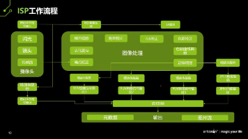

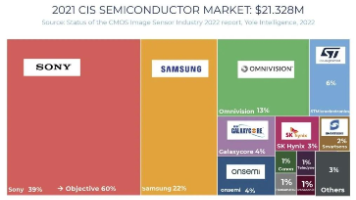
 22
22 0
0- 0


 已为社区贡献2条内容

所有评论(0)